When you write a program that simulates data from a statistical model, you should always check that the simulation code is correct. One way to do this is to generate a large simulated sample, estimate the parameters in the simulated data, and make sure that the estimates are close to the parameters in the simulation. For regression models that include CLASS variables, this task requires a bit of thought. The problem is that categorical variables can have different parameterizations, and the parameterization determines the parameter estimates.
Recently I read a published paper that included a simulation in SAS of data from a logistic model. I noticed that the parameters in the simulation code did not match the parameter estimates in the example. I was initially confused, although I figured it out eventually. This article describes the "parameterization problem" and shows how to ensure that the parameters in the simulation code match the parameter estimates for the analysis.
I have previously written about how to incorporate classification variables into simulations of regression data. If you haven't read that article, it is a good place to begin. You can also read about how to simulate data from a general linear regression model, such as a logistic regression model.
Simulated explanatory variables with a classification variable
Before demonstrating the problem, let's simulate the explanatory variables. Each simulation will use the same data and the same model but change the way that the model is parameterized. The following SAS DATA step simulates two normal variables and a categorical "treatment" variable that has three levels (Trt=1, 2, or 3). The design is balanced in the treatment variable, which means that each treatment group has the same number of observations.
data SimExplanatory; call streaminit(54321); do i = 1 to 2000; /* number in each treatment group */ do Trt = 1 to 3; /* Trt = 1, 2, and 3 */ x1 = rand('Normal'); /* x1 ~ N(0,1) */ x2 = rand('Normal'); /* x2 ~ N(0,1) */ LinCont = -1.5 + 0.4*x1 - 0.7*x2; /* offset = -1.5; params are 0.4 and -0.7 for x1 and x2 */ output; end; end; drop i; run; |
The data set contains a variable called LinCont. The LinCont variable is a linear combination of the x1 and x2 variables and a constant offset. All models will use the same offset (-1.5) and the same parameters for x1 and x2 (0.4 and -0.7, respectively).
Data for a logistic regression model with a CLASS variable
When writing a simulation of data that satisfy a regression model, most programmers assign coefficients for each level of the treatment variable. For example, you might use the coefficients {1, 2, 3}, which means that the response for the group Trt=1 gets 3 additional units of response, that the group Trt=2 gets 2 additional units, and that the group Trt=3 gets only 1 additional unit. This is a valid way to specify the model, but when you compute the regression estimates, you will discover that they are not close to the parameters in the model. The following DATA step simulates logistic data and uses PROC LOGISTIC to fit a model to the simulated data.
data LogiSim_Attempt; call streaminit(123); set SimExplanatory; /* read the explanatory variables */ array TrtCoef[3] _temporary_ (3, 2, 1); /* treatment effects */ /* a straightforward way to generate Y data from a logistic model */ eta = LinCont + TrtCoef[1]*(Trt=1) + TrtCoef[2]*(Trt=2) + TrtCoef[3]*(Trt=3); p = logistic(eta); /* P(Y | explanatory vars) */ y = rand("Bernoulli", p); /* random realization of Y */ drop eta p; run; title "Parameter Estimates Do Not Match Simulation Code"; ods select ParameterEstimates; proc logistic data=LogiSim_Attempt plots=none; class Trt; model y(event='1') = Trt x1 x2; run; |
Notice that the simulation uses the expression (Trt=1) and (Trt=2) and (Trt=3). These are binary expressions. For any value of Trt, one of the terms is unity and the others are zero.
Notice that the parameter estimates for the levels of the Trt variable do not match the parameters in the model. The model specified parameters {3, 2, 1}, but the estimates are close to {1, 0, ???}, where '???' is used to indicate that the ParameterEstimates table does not include a row for the Trt=3 level. Furthermore, the estimate for the Intercept is not close to the parameter value, which is -1.5.
I see many simulations like this. The problem is that the parameterization used by the statistical analysis procedure (here, PROC LOGISTIC) is different from the model's parameterization. The next section shows how to write a simulation so that the parameters in the simulation code and the parameter estimates agree.
The 'reference' parameterization
You can't estimate all three coefficients of the categorical variable. However, you can estimate the differences between the levels. For example, you can estimate the average difference between the Trt=1 group and the Trt=3 group. One parameterization of regression models is the "reference parameterization." In the reference parameterization, one of the treatment levels is used as a reference level and you estimate the difference between the non-reference effects and the reference effect. The Intercept parameter is the sum of the offset value and the reference effect. The following simulation code simulates data by using a reference parameterization:
data LogiSim_Ref; call streaminit(123); set SimExplanatory; /* assume reference or GLM parameterization */ array TrtCoef[3] _temporary_ (3, 2, 1); /* treatment effects */ RefLevel = TrtCoef[3]; /* use last level as reference */ eta = LinCont + RefLevel /* constant term is (Intercept + RefLevel) */ + (TrtCoef[1]-RefLevel)*(Trt=1) /* param = +2 */ + (TrtCoef[2]-RefLevel)*(Trt=2) /* param = +1 */ + (TrtCoef[3]-RefLevel)*(Trt=3); /* param = 0 */ p = logistic(eta); /* P(Y | explanatory vars) */ y = rand("Bernoulli", p); /* random realization of Y */ drop eta p; run; title "Reference Parameterization"; ods select ParameterEstimates; proc logistic data=LogiSim_Ref plots=none; class Trt / param=reference ref=LAST; /* reference parameterization */ model y(event='1') = Trt x1 x2; run; |
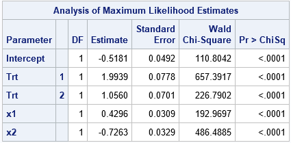
In this simulation and analysis, the constant term in the model is "Intercept + RefLevel," which is -0.5. The parameter for the Trt=1 effect is +2, which is "TrtCoef[1]-RefLevel." Similarly, the parameter for the Trt=2 effect is +1, and the parameter for Trt=3 is 0. Notice that the parameter estimates from PROC LOGISTIC agree with these values because I specified the PARAM=REFERENCE option, which tells the procedure to use the same parameterization as the simulation code.
Notice that this model is the same as the previous model because we are simply adding the RefLevel to the constant term and subtracting it from the Trt effect.
The 'effect' parameterization
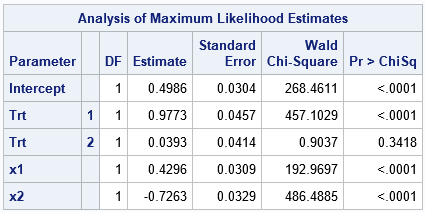
In a similar way, instead of subtracting a reference level, you can subtract the mean of the coefficients for the treatment effects. For these data, the mean of the treatment effects is (3+2+1)/3 = 2. The following simulation adds the mean to the constant term and subtracts it from the Trt effects. This is the "effect parameterization":
data LogiSim_Effect; call streaminit(123); set SimExplanatory; array TrtCoef[3] _temporary_ (3, 2, 1); /* treatment effects */ /* assume effect parameterization, which is equivalent to using deviations from the mean: array TrtDev[3] _temporary_ (+1, 0, -1); */ MeanTrt = 2; /* mean = (3+2+1) / 3 */ eta = LinCont + MeanTrt /* est intercept = (Intercept + MeanTrt) */ + (TrtCoef[1]-MeanTrt)*(Trt=1) /* param = +1 */ + (TrtCoef[2]-MeanTrt)*(Trt=2) /* param = 0 */ + (TrtCoef[3]-MeanTrt)*(Trt=3); /* param = -1 */ p = logistic(eta); /* P(Y | explanatory vars) */ y = rand("Bernoulli", p); /* random realization of Y */ drop eta p; run; title "Effect Parameterization"; ods select ParameterEstimates; proc logistic data=LogiSim_effect plots=none; class Trt / param=effect ref=LAST; model y(event='1') = Trt x1 x2; run; |
In this simulation and analysis, the constant term in the model is "Intercept + MeanTrt," which is 0.5. The parameters for the Trt levels are {+1, 0, -1}. Notice that the PROC LOGISTIC call uses the PARAM=EFFECT option, which tells the procedure to use the same effect parameterization. Consequently, the parameter estimates are close to the parameter values. (These are the same parameter estimates as in the first example, since PROC LOGISTIC uses the effect parameterization by default.)
If you use 0 as an offset value, then the Intercept parameter equals the mean effect of the treatment variable, which leads to a nice interpretation when there is only one classification variable and no interactions.
Summary
This article shows how to write the simulation code (the equation of the linear predictor) so that it matches the parameterization used to analyze the data. This article uses PROC LOGISTIC, but you can use the same trick for other procedures and analyses. When the simulation code and the analysis use the same parameterization of classification effects, it is easier to feel confident that your simulation code correctly simulates data from the model that you are analyzing.

2 Comments
Hello Rick, when I run my first regression models I spent a bunch of time on understanding the difference between the coding schemes. You wrote several articles on that and which procs offer choices i this regard. I learned that its correct appliance is fundamental when wanting to construct effect statements.
But if I remember correctly the effect coding has the grand mean but not weighted.
You are correct. Thanks for the correction. I have deleted the incorrect sentence in the post.