I was recently asked about how to interpret the output from the COLLIN (or COLLINOINT) option on the MODEL statement in PROC REG in SAS. The example in the documentation for PROC REG is correct but is somewhat terse regarding how to use the output to diagnose collinearity and how to determine which variables are collinear. This article uses the same data but goes into more detail about how to interpret the results of the COLLIN and COLLINOINT options.
An overview of collinearity in regression
Collinearity (sometimes called multicollinearity) involves only the explanatory variables. It occurs when a variable is nearly a linear combination of other variables in the model. Equivalently, there a set of explanatory variables that is linearly dependent in the sense of linear algebra. (Another equivalent statement is that the design matrix and the X`X matrices are not full rank.)
For example, suppose a model contains five regressor variables and the variables are related by X3 = 3*X1 - X2 and X5 = 2*X4;. In this case, there are two sets of linear relationships among the regressors, one relationship that involves the variables X1, X2, and X3, and another that involves the variables X4 and X5. In practice, collinearity means that a set of variables are almost linearly combinations of each other. For example, the vectors u = X3 - 3*X1 + X2 and v = X5 - 2*X4; are close to the zero vector.
Unfortunately, the words "almost" and "close to" are difficult to quantify. The COLLIN option on the MODEL statement in PROC REG provides a way to analyze the design matrix for potentially harmful collinearities.
Why should you avoid collinearity in regression?
The assumptions of ordinary least square (OLS) regression are not violated if there is collinearity among the independent variables. OLS regression still provides the best linear unbiased estimates of the regression coefficients.
The problem is not the estimates themselves but rather the variance of the estimates. One problem caused by collinearity is that the standard errors of those estimates will be big. This means that the predicted values, although the "best possible," will have wide prediction limits. In other words, you get predictions, but you can't really trust them.
A second problem concerns interpretability. The sign and magnitude of a parameter estimate indicate how the dependent variable changes due to a unit change of the independent variable when the other variables are held constant. However, if X1 is nearly collinear with X2 and X3, it does not make sense to discuss "holding constant" the other variables (X2 and X3) while changing X1. The variables necessarily must change together. Collinearities can even cause some parameter estimates to have "wrong signs" that conflict with your intuitive notion about how the dependent variable should depend on an independent variable.
A third problem with collinearities is numerical rather than statistical. Strong collinearities cause the cross-product matrix (X`X) to become ill-conditioned. Computing the least squares estimates requires solving a linear system that involves the cross-product matrix. Solving an ill-conditioned system can result in relatively large numerical errors. However, in practice, the statistical issues usually outweigh the numerical one. A matrix must be extremely ill-conditioned before the numerical errors become important, whereas the statistical issues are problematic for moderate to large collinearities.
How to interpret the output of the COLLIN option?
The following example is from the "Collinearity Diagnostics" section of the PROC REG documentation. Various health and fitness measurements were recorded for 31 men, such as time to run 1.5 miles, the resting pulse, the average pulse rate while running, and the maximum pulse rate while running. These measurements are used to predict the oxygen intake rate, which is a measurement of fitness but is difficult to measure directly.
data fitness; input Age Weight Oxygen RunTime RestPulse RunPulse MaxPulse @@; datalines; 44 89.47 44.609 11.37 62 178 182 40 75.07 45.313 10.07 62 185 185 44 85.84 54.297 8.65 45 156 168 42 68.15 59.571 8.17 40 166 172 38 89.02 49.874 9.22 55 178 180 47 77.45 44.811 11.63 58 176 176 40 75.98 45.681 11.95 70 176 180 43 81.19 49.091 10.85 64 162 170 44 81.42 39.442 13.08 63 174 176 38 81.87 60.055 8.63 48 170 186 44 73.03 50.541 10.13 45 168 168 45 87.66 37.388 14.03 56 186 192 45 66.45 44.754 11.12 51 176 176 47 79.15 47.273 10.60 47 162 164 54 83.12 51.855 10.33 50 166 170 49 81.42 49.156 8.95 44 180 185 51 69.63 40.836 10.95 57 168 172 51 77.91 46.672 10.00 48 162 168 48 91.63 46.774 10.25 48 162 164 49 73.37 50.388 10.08 67 168 168 57 73.37 39.407 12.63 58 174 176 54 79.38 46.080 11.17 62 156 165 52 76.32 45.441 9.63 48 164 166 50 70.87 54.625 8.92 48 146 155 51 67.25 45.118 11.08 48 172 172 54 91.63 39.203 12.88 44 168 172 51 73.71 45.790 10.47 59 186 188 57 59.08 50.545 9.93 49 148 155 49 76.32 48.673 9.40 56 186 188 48 61.24 47.920 11.50 52 170 176 52 82.78 47.467 10.50 53 170 172 ; proc reg data=fitness plots=none; model Oxygen = RunTime Age Weight RunPulse MaxPulse RestPulse / collin; ods select ParameterEstimates CollinDiag; ods output CollinDiag = CollinReg; quit; |
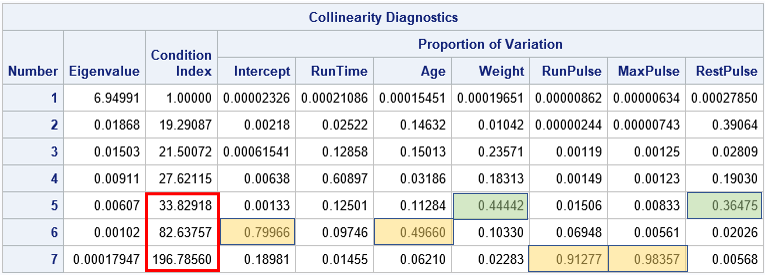
The output from the COLLIN option is shown. I have added some colored rectangles to the output to emphasize how to interpret the table. To determine collinearity from the output, do the following:
- Look at the "Condition Index" column. Large values in this column indicate potential collinearities. Many authors use 30 as a number that warrants further investigation. Other researchers suggest 100. Most researchers agree that no single number can handle all situations.
- For each row that has a large condition index, look across the columns in the "Proportion of Variation" section of the table. Identify cells that have a value of 0.5 or greater. The columns of these cells indicate which variables contribute to the collinearity. Notice that at least two variables are involved in each collinearity, so look for at least two cells with large values in each row. However, there could be three or more cells that have large values. "Large" is relative to the value 1, which is the sum of each column.
Let's apply these rules to the output for the example:
- If you use 30 as a cutoff value, there are three rows (marked in red) whose condition numbers exceed the cutoff value. They are rows 5, 6, and 7.
- For the 5th row (condition index=33.8), there are no cells that exceed 0.5. The two largest cells (in the Weight and RestPulse columns) indicate a small near-collinearity between the Weight and RestPulse measurements. The relationship is not strong enough to worry about.
- For the 6th row (condition index=82.6), there are two cells that are 0.5 or greater (rounded to four decimals). The cells are in the Intercept and Age columns. This indicates that the Age and Intercept terms are nearly collinear. Collinearities with the intercept term can be hard to interpret. See the comments at the end of this article.
- For the 7th row (condition index=196.8), there are two cells that are greater than 0.5. The cells are in the RunPulse and MaxPulse columns, which indicates a very strong linear relationship between these two variables.
Your model has collinearities. Now what?
After you identify the cause of the collinearities, what should you do? That is a difficult and controversial question that has many possible answers.
- Perhaps the simplest solution is to use domain knowledge to omit the "redundant" variables. For example, you might want to drop MaxPulse from the model and refit. However, in this era of Big Data and machine learning, some analysts want an automated solution.
- You can use dimensionality reduction and an (incomplete) principal component regression. (This link also discussed partial least squares (PLS).)
- You can use a biased estimation technique such as ridge regression, which allows bias but reduces the variance of the estimates.
- Some practitioners use variable selection techniques to let the data decide which variables to omit from the model. However, be aware that different variable-selection methods might choose different variables from among the set of nearly collinear variables.
Should you center the data before performing the collinearity check?
Equally controversial is the question of whether to include the intercept term as a variable when running the collinearity diagnostics. The COLLIN option in PROC REG includes the intercept term among the variables to be analyzed for collinearity. The COLLINOINT option excludes the intercept term and, more importantly, centers the data by subtracting the mean of each column in the data matrix. Which should you use? Here are two opinions that I found:
- Do not center the data (Use the intercept term): Belsley, Kuh, and Welsch (Regression Diagnostics, 1980, p. 120) state that centering is "inappropriate in the event that [the design matrix]contains a constant column." They go on to say (p. 157) that "centering the data [when the model has an intercept term]can mask the role of the constant in any near dependencies and produce misleading diagnostic results." These quotes strongly favor using the COLLIN option, which analyzes exactly the design matrix that is used to construct the parameter estimates for the regression.
- Center the data (Do not use the intercept term): If the intercept is outside of the data range, Freund and Littell (SAS System for Regression, 3rd Ed, 2000) argue that including the intercept term in the collinearity analysis is not always appropriate. "The intercept is an estimate of the response at the origin, that is, where all independent variables are zero. .... [F]or most applications the intercept represents an extrapolation far beyond the reach of the data. For this reason, the inclusion of the intercept in the study of multicollinearity can be useful only if the intercept has some physical interpretation and is within reach of the actual data space." For the example data, it is impossible for a person to have zero age, weight, or pulse rate, therefore I suspect Freund and Little would recommend using the COLLINOINT option for these data. Remember that the COLLINOINT option centers the data, so you are performing collinearity diagnostics on a different data matrix than is used to construct the regression estimates.
So what should you do if the experts disagree? Well, SAS provides both options, but I usually defer to the math. Although I am reluctant to contradict Freund and Littell (both widely published experts and Fellows of the American Statistical Association), the mathematics of the collinearity analysis seems to favor the opinion of Belsley, Kuh, and Welsch, who argue for analyzing the same design matrix that is used for the regression estimates. This means using the COLLIN option. I have written a separate article that investigates this issue in more detail.
Do you have an opinion on this matter? Leave a comment.

11 Comments
I did my dissertation on this! And this is a very good summary., as usual.
My view is that Belsley is right about the intercept. In very non-techie terms, excluding the intercept just pushes the collinearity somewhere else.I remember studying the math, but have forgotten the details (I suppose I could go read my dissertation......but who does that?)
One thing I was surprised not to see mentioned is partial least squares regression which, to me, is better than principal component regression but serves a similar purpose. What are your thoughts on that?
If you follow the link that I gave for PC regression, you will see a paragraph on PLS.
I think that Statistical Model Development is primarily about solving a "business / research" decision problem and as such, the strategic / tactical model development choices should be guided more by the problem domain, data quality and the data structures and less by mathematics. The issue of including an intercept term in a model should be based on the practical interpretation. The fuzzy alternative to this dilemma would be to do both and then compare the resultant two models w.r.t. usefulness and implementation. Perhaps this is a good example of the perils of unsupervised machine learning methodologies ??? Completely Autonomous Cars ("Baby You Can Drive My Car" ) followed by Completely Autonomous Statisticians?
I agree with what you say about model development, but that is not the issue here. The question is about collinearity diagnostics. In a model THAT HAS AN INTERCEPT, some people argue that you can drop the intercept as a column in the design matrix WHEN YOU RUN COLLINEARITY DIAGNOSTICS. Others (including myself), argue that you need to keep the column when you assess collinearity.
IF the inclusion of the intercept term in the model is valid / makes "business" sense and one is evaluating that specific model where colinearity within the underlying data may impact the application of that model, then I would consider what it means for there to be collinearity within the design matrix that includes an intercept as opposed to collinearity within a corresponding design matrix / data set that does not include the intercept term. In this case, the inclusion of the intercept term in the collinearity analysis may assist in the diagnosis of collinearity between the "explanatory" variables in the model and the evaluation of the data quality issues w.r.t. the statistical model being developed and evaluated. However, the numerical computations on the design matrix that are required to estimate the model parameters and which are also used to evaluate the degree of collinearity and thus the stability of the model, should be used with caution and as a guide to possibly modifying the model. You certainly CAN drop the intercept term but the question is which model is better suited to solving the decision problem and thus the question is: SHOULD you drop the intercept term? Evaluation of the impact of including and excluding the intercept term during the Collinearity Diagnosis as well as the evaluation of the impact on the statistical model are joined at the hip
Thanks for the comment. As you say, an intercept term should be included when it makes sense. If there is a collinearity between the Intercept and another variable (Z), I would look at whether to keep Z in the model. I would not suggest dropping the intercept term.
Rick,
Another option CORRB also can help judge the collinearity .
I have a question.As you said:
" Collinearities can even cause some parameter estimates to have "wrong signs" that conflict with your intuitive notion"
Does that mean ALL the parameter estimator must be positive or negative ?
I think you mean the COVB option. The standard errors of the parameter estimates are the diagonal elements of the COVB matrix.
No, it does not mean that all estimates have to have the same sign. The statement is merely a comment about solutions for X`X when the matrix is nearly singular. Suppose you think that Y should be positively related to X1 and X2. When only X1 is in the model, the model is Y = 10*X1. What happens if you add X2? You might hope for Y = 5*X1 + 5*X2, but an equally valid solution is Y = 12*X1 - 2*X2. This equation makes it look like Y is negatively related to Y, but it isn't. Instead the collinearity is causing the coefficient of X2 to have the "wrong sign."
Rick,
proc reg data=fitness plots=none;
model Oxygen = RunTime Age Weight RunPulse MaxPulse RestPulse / corrb;
quit;
I can get the following:
Variables Intercept RunTime Age Weight RunPulse MaxPulse RestPulse
Intercept 1.0000 0.1610 -0.7285 -0.2632 0.1889 -0.4919 -0.1806
RunTime 0.1610 1.0000 -0.3696 -0.2104 -0.1963 0.0881 -0.4297
Age -0.7285 -0.3696 1.0000 0.1875 -0.1006 0.2629 0.2259
Weight -0.2632 -0.2104 0.1875 1.0000 0.1474 -0.1842 0.1054
RunPulse 0.1889 -0.1963 -0.1006 0.1474 1.0000 -0.9140 -0.0966
MaxPulse -0.4919 0.0881 0.2629 -0.1842 -0.9140 1.0000 0.0380
RestPulse -0.1806 -0.4297 0.2259 0.1054 -0.0966 0.0380 1.0000
MaxPulse V.S. RunPulse = -0.9140
Age V.S. Intercept = -0.7285
The same result as yours .
It is related. The collinearities in my article are between data vectors. The CORRB matrix is an estimate of the correlations between the regression coefficients. If you have large collinearities between X1 and X2, there will be strong correlations between the coefficients of X1 and X2. However, the collinearity diagnostics in this article provide a step-by-step algorithm for detecting collinearities in the data. I am not aware of a similar algorithm for the CORRB matrix.
Pingback: Visualize collinearity diagnostics - The DO Loop