Longitudinal data are used in many health-related studies in which individuals are measured at multiple points in time to monitor changes in a response variable, such as weight, cholesterol, or blood pressure. There are many excellent articles and books that describe the advantages of a mixed model for analyzing longitudinal data. Recently, I encountered an introductory article that summarizes the essential issues in a little more than five pages! You can download the article for free: "A Primer in Longitudinal Data Analysis", by G. Fitzmaurice and C. Ravichandran (2008), Circulation, 118(19), p. 2005-2010.
The article analyzes a set of longitudinal data in two ways. First, the authors use a traditional linear model to perform an "analysis of response profiles." Then, the authors discuss how a mixed model can correct some of the deficiencies of the analysis. This blog post analyzes the same data by using PROC GLM in SAS. A second blog post analyzes the same data by using PROC MIXED in SAS.
Longitudinal Data: Treatment of lead-exposed children
Fitzmaurice and C. Ravichandran analyze data for a randomized trial involving toddlers who were exposed to high levels of lead. The article analyzes a subset of 100 children. Half the children were given a treatment (called succimer) and the other half were given a placebo. The blood lead levels were measured for each child at baseline (week 0), week 1, week 4, and week 6. The main scientific question is "whether the two treatment groups differ in their patterns of change from baseline in mean blood lead levels" (p. 2006).
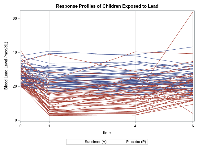
The children in the subset were measured at all four time points. There are no missing values or mistimed measurements. (This situation is fairly unusual in longitudinal data, which is often plagued by missed appointments or individuals who leave the study.) The following "spaghetti plot" shows the individual measurements for the 100 children at each time point. Each line represents a child. Blue lines indicate that the child was in the placebo group; red lines indicate the experimental group that was given succimer.
Analysis of response profiles
In an analysis of response profiles, you compare the mean response-by-time profile for the treatment and placebo groups. You can visualize the mean response over time for each group by using the VBAR statement in PROC SGPLOT. The following graph shows the mean value and standard error for each time point for each treatment group:
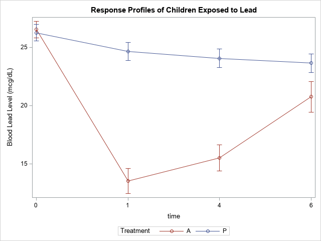
If the treatment is ineffective, the line segments for the two treatment groups will be approximately parallel. The graph shows that this is not that case for these data. The visualization indicates that the mean blood-lead value for the treatment group (Treatment='A') is lower than for the placebo group at 1 and 4 weeks.
You can use PROC GLM to confirm that these differences are statistically significant and to estimate the effect that taking succimer had on the mean blood-lead level:
proc glm data=tlc; class Time(ref='0') Treatment(ref='P'); model y = Treatment Time Treatment*Time / solution; output out=GLMOut Predicted=Pred; quit; |
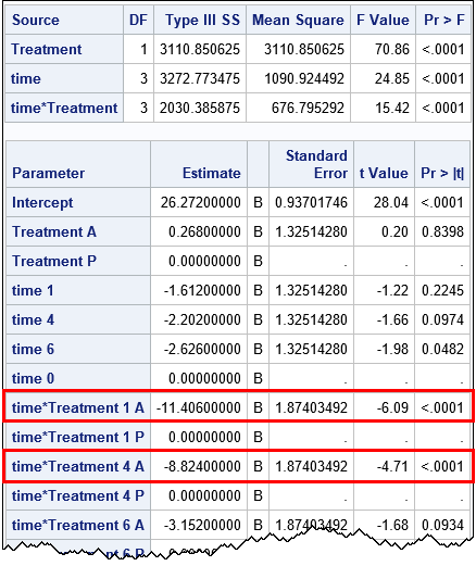
According to the Type 3 statistics, all three effects in the model are significant. The parameter estimates (outlined in red) indicate that the mean blood-lead level for children in the Treatment='A' group is 11.4 mcg/dL lower than the children in the placebo group after 1 week. Similarly, after four weeks the mean of the experimental group is 8.8 mcg/dL lower than the placebo group. These are both significant differences, so the response-profile analysis provides a positive answer to the research question: the profile for the treatment group is lower than the placebo group.
Advantages and disadvantages of the analysis of response profiles
As discussed in Fitzmaurice and Ravichandran (2008), the analysis of the response profile has several advantages:
- It is familiar to researchers who have experience with ANOVA.
- It does not require any advanced statistical modeling , such as modeling the covariance of the repeated measurements.
However, this simple method suffers from several statistical problems:
- Longitudinal data do not satisfy the assumptions of linear regression and ANOVA. Because the data contains repeated measures from the same individuals, the residual errors are neither independent nor do they have constant variance (homoscedastic).
- Some participants in a study might miss an appointment or drop out of the study. Others might be measured at time points that were not part of the design (for example, at 2 or 3 weeks). These two problems are known as incomplete data and mistimed measurements, respectively. Although the first can be handled by using an unbalanced ANOVA, the second is a problem that does not have a simple solution within an ANOVA model that uses discrete time points.
- The response-profile analysis does not enable you to model each individual's response as a function of time.
Prediction of individual response profiles
The inability to model individual trajectories is often the reason that researchers abandon the response-profile analysis in favor of a more complicated mixed model. To be clear, the GLM model can make predictions, but the predicted values for every child in the placebo group are the same. Similarly, the predicted values for every child in the experimental group are the same. This is shown in the following panel of graphs, which shows the predicted response curves for six children in the study, three from each treatment group.
/* Look at predictions for each individual. They are identical! */ proc sort data=GLMOut(where=(ID in (1,2,4,5,6,7))) out=GLMSubset; by Treatment ID; run; title2 "Fixed Effect Model"; proc sgpanel data=GLMSubset dattrmap=Order; panelby Treatment ID; scatter x=Time y=y / group=Treatment attrid=Treat; series x=Time y=Pred / group=Treatment attrid=Treat; run; |
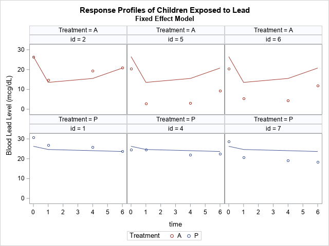
Notice that the predicted responses are the same across the top row (ID=2, 5, and 6). These children were all in the experimental group. Although the predicted values seem to fit the actual observed response for ID=2, the predicted responses for ID=5 and ID=6 are much higher than the observed responses. Although the predicted response is the best prediction for an "average patient," it does not account for individual differences in the study participants.
The same is true for the patients in the placebo group, three of which are plotted in the second row. The predicted values are "too low" for ID=1 and are "too high" for ID=4.
If modeling the individual profiles is important, then clearly this method is not sufficient. If you want to model the individual profiles, you can use a linear mixed model. The mixed model also addresses other deficiencies of the response-profile analysis. The mixed model is described in the next blog post.
You can download the SAS code and data for the response-profile analysis.
Further reading
This blog post is a brief summary of the article "A Primer in Longitudinal Data Analysis" (Fitzmaurice and Ravichandran, 2008). See the article for more details. Also, these data and these ideas are also discussed in the book Applied Longitudinal Analysis (2011, 2nd Ed) by G. Fitzmaurice, N. Laird, and J. Ware. You can download data (and SAS programs) from the book at the book's web site.

3 Comments
Pingback: Longitudinal data: The mixed model - The DO Loop
Dear Dr Wicklin,
thanks for this insightful post.
I would like to know if this type of analysis is suitable for longitudinal data on a single cohort of students. I am analysing new entrants in graduate programs in Brazil of the 2013 cohort and observing their pathways along 5 years. So I am interested in looking at conclusion and dropout rates by areas of study and other groups.
Best regards,
Alice.
The response-profile model has limitations. See the section "Advantages and disadvantages of the analysis of response profiles." Mixed models were created to address those limitations. See the follow-up article "Longitudinal data: The mixed model."