One of the strengths of the SAS/IML language is its flexibility. Recently, a SAS programmer asked how to generalize a program in a previous article. The original program solved one optimization problem. The reader said that she wants to solve this type of problem 300 times, each time using a different set of parameters. Essentially, she wants to loop over a set of parameter values, solve the corresponding optimization problem, and save each solution to a data set.
Yes, you can do this in SAS/IML, and the technique is not limited to solving a series of optimization problems. Any time you have a parameterized family of problems, you can implement this idea. First, you figure out how to solve the problem for one set of parameters, then you can loop over many sets of parameters and solve each problem in turn.
Solve the problem one time
As I say in my article, "Ten tips before you run an optimization," you should always develop and debug solving ONE problem before you attempt to solve MANY problems. This section describes the problem and solves it for one set of parameters.
For this article, the goal is to find the values (x1, x2) that maximize a function of two variables:
F(x1, x2; a b) = 1 – (x1 – a)2 – (x2 – b)2 +
exp(–(x12 + x22)/2);
The function has two parameters, (a, b), which are not involved in the optimization. The function is a sum of two terms: a quadratic function and an exponentially decreasing function that looks like the bivariate normal density.
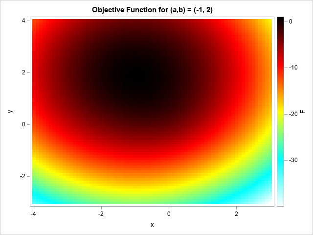
Because the exponential term rapidly approaches zero when (x1, x2) moves away from the origin, this function is a perturbation of a quadratic function. The maximum will occur somewhat close to the value (x1, x2) = (a, b), which is the value for which the quadratic term is maximal. The following graph shows a contour plot for the function when (a, b) = (-1, 2). The maximum value occurs at approximately (x1, x2) = (-0.95, 1.9).
The following program defines the function in the SAS/IML language. In the definition, the parameters (a, b) are put in the GLOBAL statement because they are constant during each optimization. The SAS/IML language provides several nonlinear optimization routines. This program uses Newton-Raphson optimizer to solve the problem for (a, b) = (-1, 2).
proc iml; start Func(x) global (a, b); return 1 - (x[,1] - a)##2 - (x[,2] - b)##2 + exp(-0.5*(x[,1]##2 + x[,2]##2)); finish; a = -1; b = 2; /* set GLOBAL parameters */ /* test functions for one set of parameters */ opt = {1, /* find maximum of function */ 2}; /* print a little bit of output */ x0 = {0 0}; /* initial guess for solution */ call nlpnra(rc, result, "Func", x0, opt); /* find maximal solution */ print result[c={"x1" "x2"}]; |
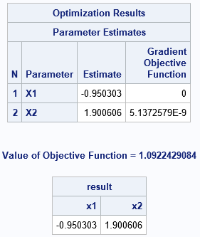
As claimed earlier, when (a, b) = (-1, 2), the maximum value of the function occurs at approximately (x1, x2) = (-0.95, 1.9).
Solve the problem for many parameters
After you have successfully solved the problem for one set of parameters, you can iterate over a sequence of parameters. The following DATA step specifies five sets of parameters, but it could specify 300 or 3,000. These parameters are read into a SAS/IML matrix. When you solve a problem many times in a loop, it is a good idea to suppress any output. The SAS/IML program suppresses the tables and iteration history for each optimization step and saves the solution and the convergence status:
/* define a set of parameter values */ data Params; input a b; datalines; -1 2 0 1 0 4 1 0 3 2 ; proc iml; start Func(x) global (a, b); return 1 - (x[,1] - a)##2 - (x[,2] - b)##2 + exp(-0.5*(x[,1]##2 + x[,2]##2)); finish; /* read parameters into a matrix */ varNames = {'a' 'b'}; use Params; read all var varNames into Parms; close; /* loop over parameters and solve problem */ opt = {1, /* find maximum of function */ 0}; /* no print */ Soln = j(nrow(Parms), 2, .); returnCode = j(nrow(Parms), 1, .); do i = 1 to nrow(Parms); /* assign GLOBAL variables */ a = Parms[i, 1]; b = Parms[i, 2]; /* For now, use same guess for every parameter. */ x0 = {0 0}; /* initial guess for solution */ call nlpnra(rc, result, "Func", x0, opt); returnCode[i] = rc; /* save convergence status and solution vector */ Soln[i,] = result; end; print Parms[c=varNames] returnCode Soln[c={x1 x2} format=Best8.]; |
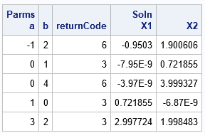
The output shows the parameter values (a,b), the status of the optimization, and the optimal solution for (x1, x2). The third column (returnCode) has the value 3 or 6 for these optimizations. You can look up the exact meaning of the return codes, but the main thing to remember is that a positive return code indicates a successful optimization. A negative return code indicates that the optimization terminated without finding an optimal solution. For this example, all five problems were solved successfully.
Choosing an initial guess based on the parameters
If the problem is not solved successfully for a certain parameter value, it might be that the initial guess was not very good. It is often possible to approximate the objective function to obtain a good initial guess for the solution. This not only helps ensure convergence, but it often improves the speed of convergence. If you want to solve 300 problems, having a good guess will speed up the total time.
For this example, the objective functions are a perturbation of a quadratic function. It is easy to show that the quadratic function has an optimal solution at (x1, x2) = (a, b), and you can verify from the previous output table that the optimal solutions are close to (a, b). Consequently, if you use (a, b) as an initial guess, rather than a generic value like (0, 0), then each problem will converge in only a few iterations. For this problem, the GetInitialGuess function return (a,b), but in general the function would return a function of the parameter or even solve a simpler set of equations.
/* Choose an initial guess based on the parameters. */ start GetInitialGuess(Parms); return Parms; /* for this problem, the solution is near (x1,x2)=(a,b) */ finish; do i = 1 to nrow(Parms); /* assign GLOBAL variables */ a = Parms[i, 1]; b = Parms[i, 2]; /* Choose an initial guess based on the parameters. */ x0 = GetInitialGuess(Parms[i,]); /* initial guess for solution */ call nlpnra(rc, result, "Func", x0, opt); returnCode[i] = rc; Soln[i,] = result; end; print Parms[c=varNames] returnCode Soln[c={x1 x2} format=Best8.]; |
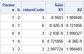
The solutions and return codes are similar to the previous example. You can see that changing the initial guess changes the convergence status and slightly changes the solution values.
For this simple problem, choosing a better initial guess provides only a small boost to performance. If you use (0,0) as an initial guess, you can solve 3,000 problems in about 2 seconds. If you use the GetInitialGuess function, it takes about 1.8 seconds to solve the same set of optimizations. For other problems, providing a good initial guess might be more important.
In conclusion, the SAS/IML language makes it easy to solve multiple optimization problems, where each problem uses a different set of parameter values. To improve convergence, you can sometimes use the parameter values to compute an initial guess.

2 Comments
My friend and colleague, Rob Pratt, sent me this PROC OPTMODEL code that performs the same optimizations but uses the COFOR statement in PROC OPTMODEL to solve the problems in parallel on multiple threads. Very nice!
For SAS customers who have access to SAS Viya 3.5, you can solve this problem by using BY-group processing in the runOptmodel action: