Binning transforms a continuous numerical variable into a discrete variable with a small number of values. When you bin univariate data, you define cut point that define discrete groups. I've previously shown how to use PROC FORMAT in SAS to bin numerical variables and give each group a meaningful name such as 'Low,' 'Medium,' and 'High.' This article uses PROC HPBIN to create bins that are assigned numbers. If you bin the data into k groups, the groups have the integer values 1, 2, 3, ..., k. Missing values are put into the zeroth group.
There are two popular ways to choose the cut points. You can use evenly spaced points, or you can use quantiles of the data. If you use evenly spaced cut points (as in a histogram), the number of observations in each bin will usually vary. Using evenly spaced cut points is called the "bucket binning" method. Alternatively, if you use quantiles as cut points (such as tertiles, quartiles, or deciles), the number of observations in each bin tend to be more balanced. This article shows how to use PROC HPBIN in SAS to perform bucket binning and quantile binning. It also shows how to use the CODE statement in PROC HPBIN to create a DATA step that uses the same cut points to bin future observations.
Create sample data
The following statements create sample data from the Sashelp.Heart data. An ID variable is added to the data so that you can identify each observation. A call to PROC MEANS produces descriptive statistics about two variables: Cholesterol and Systolic blood pressure.
data Heart; format PatientID Z5.; set Sashelp.Heart(keep=Sex Cholesterol Systolic); PatientID = 10000 + _N_; run; proc means data=Heart nolabels N NMISS Min Max Skewness; var Cholesterol Systolic; run; |
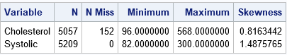
The output shows the range of the data for each variable. It also shows that the Cholesterol variable has 152 missing values. If your analysis requires nonmissing observations, you can use PROC HPIMPUTE to replace the missing values. For this article, I will not replace the missing values so that you can see how PROC HPBIN handles missing values.
Each variable has a skewed distribution, as indicated by the values of the skewness statistic. This usually indicates that equal-length binning will result in bins in the tail of the distribution that have only a few observations.
Use PROC HPBIN to bin data into equal-length bins
A histogram divides the range of the data by using k evenly spaced cutpoints. The width of each bin is (Max – Min) / k. PROC HPBIN enables you to create new variables that indicate to which bin each observation belongs. You can use the global NUMBIN= option on the PROC HPBIN statement to set the default number of bins for each variable. You can use the INPUT statement to specify which variables to bin. You can override the default number of bins by using the NUMBIN= option on any INPUT statement.
Suppose that you want to bin the Cholesterol data into five bins and the remaining variables into three bins.
- The range of the Cholesterol data is [96, 568], so the width of the five bins that contain nonmissing values will be 94.4.
- The range of the Systolic data is [82, 300], so the width of the three bins will be 72.66.
The following call to PROC HPBIN bins the variables. The output data set, HeartBin, contains the bin numbers for each observation.
/* equally divide the range each variable (bucket binning) */ proc hpbin data=Heart output=HeartBin numbin=3; /* global NUMBIN= option */ input Cholesterol / numbin=5; /* override global NUMBIN= option */ input Systolic; id PatientID Sex; run; |
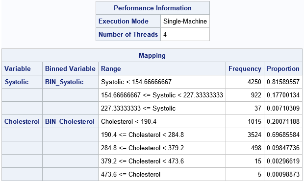
Part of the output from PROC HPBIN is shown. (You can suppress the output by using the NOPRINT option.) The first table shows that PROC HPBIN used four threads on my PC to compute the results in parallel. The second table summarizes the transformation that bins the data. For each variable, the second column gives the names of the binned variables in the OUTPUT= data set. The third column shows the cutpoints for each bin. The Frequency and Proportion column show the frequency and proportion (respectively) of observations in each bin. As expected for these skewed variables, bins in the tail of each variable contain very few observations (less than 1% of the total).
The OUTPUT= option creates an output data set that contains the indicator variables for the bins. You can use PROC FREQ to enumerate the bin values and (again) count the number of observations in each bin:
proc freq data=HeartBin; tables BIN_Cholesterol BIN_Systolic / nocum; run; |
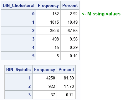
Notice that the Cholesterol variable was split into six bins even though the syntax specified NUMBIN=5. If a variable contains missing values, a separate bin is created for them. In this case, the zeroth bin contains the 152 missing values for the Cholesterol variable.
Bucket binning divides the range of the variables into equal-width intervals. For long-tailed data, the number of observations in each bin might vary widely, as for these data. The next section shows an alternative binning strategy in which the width of the bins vary and each bin contains approximately the same number of observations.
Use PROC HPBIN to bin data by using quantiles
You can use evenly-spaced quantiles as cutpoints in an attempt to balance the number of observations in the bins. However, if the data are rounded or have duplicate values, the number of observations in each bin can still vary. PROC HPBIN has two ways methods for quantile binning. The slower method (the QUANTILE option) computes cutpoints based on the sample quantiles and then bins the observations. The faster method (the PSEUDO_QUANTILE option) uses approximate quantiles to bin the data. The following call uses the PSEUDO_QUANTILE option to bin the data into approximately equal groups:
/* bin by quantiles of each variable */ proc hpbin data=Heart output=HeartBin numbin=3 pseudo_quantile; input Cholesterol / numbin=5; /* override global NUMBIN= option */ input Systolic; /* use global NUMBIN= option */ id PatientID Sex; code file='C:/Temp/BinCode.sas'; /* generate scoring code */ run; |
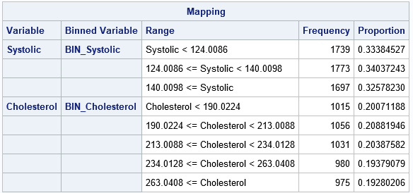
The output shows that the number of observations in each bin is more balanced. For the Systolic variable, each bin has between 1,697 and 1,773 observations. For the Cholesterol variable, each bin contains between 975 and 1,056 observations. Although not shown in the table, the BIN_Cholesterol variable also contains a bin for the 152 missing values for the Cholesterol variable.
Use PROC HPBIN to write DATA step code to bin future observations
In the previous section, I used the CODE statement to specify a file that contains SAS DATA step code that can be used to bin future observations. The statements in the BinCode.sas file are shown below:
***************** BIN_Systolic ********************; length BIN_Systolic 8; if missing(Systolic) then do; BIN_Systolic = 0; end; else if Systolic < 124.0086 then do; BIN_Systolic = 1; end; else if 124.0086 <= Systolic < 140.0098 then do; BIN_Systolic = 2; end; else if 140.0098 <= Systolic then do; BIN_Systolic = 3; end; ***************** BIN_Cholesterol ********************; length BIN_Cholesterol 8; if missing(Cholesterol) then do; BIN_Cholesterol = 0; end; else if Cholesterol < 190.0224 then do; BIN_Cholesterol = 1; end; else if 190.0224 <= Cholesterol < 213.0088 then do; BIN_Cholesterol = 2; end; else if 213.0088 <= Cholesterol < 234.0128 then do; BIN_Cholesterol = 3; end; else if 234.0128 <= Cholesterol < 263.0408 then do; BIN_Cholesterol = 4; end; else if 263.0408 <= Cholesterol then do; BIN_Cholesterol = 5; end; |
You can see from these statements that the zeroth bin is reserved for missing values. Nonmissing values will be split into bins according to the approximate tertiles (NUMBIN=3) or quintiles (NUMBIN=5) of the training data.
The following statements show how to use the file that was created by the CODE statement. New data is contained in the Patients data set. Simply use the SET statement and the %INCLUDE statement to bin the new data, as follows:
data Patients; length Sex $6; input PatientID Sex Systolic Cholesterol; datalines; 13021 Male 96 . 13022 Male 148 242 13023 Female 144 217 13024 Female 164 376 13025 Female . 248 13026 Male 190 238 13027 Female 158 326 13028 Female 188 266 ; data MakeBins; set Patients; %include 'C:/Temp/BinCode.sas'; /* include the binning statements */ run; /* Note: HPBIN puts missing values into bin 0 */ proc print data=MakeBins; run; |
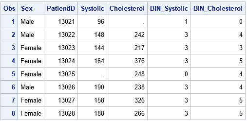
The input data can contain other variables (PatientID, Sex) that are not binned. However, the data should contain the Systolic and Cholesterol variables because the statements in the BinCode.sas file refer to those variables.
Summary
In summary, you can use PROC HPBIN in SAS to create a new discrete variable by binning a continuous variable. This transformation is common in machine learning algorithms. Two common binning methods include bucket binning (equal-length bins) and quantile binning (unequal-length bins). Missing values are put into their own bin (the zeroth bin). The CODE statement in PROC HPBIN enables you to write DATA step code that you can use to bin future observations.

8 Comments
Thank you very much, this is very useful; as far as I know the first blog entry dealing with HPBIN !
This is nicely illustrative of HPBIN.
But one question is when. if ever, binning is a good idea.
Binning an IV increases type I and type II error and introduces a kind of magical thinking. I wrote a blog post showing, graphically, why this is a bad idea. rapt attention or astonishment at something awesomely mysterious or new to one's experience and Frank Harrell in Regression Modeling Strategies (an excellent book, even if he uses R) lists (I think) 11 problems with this. Better to use splines via ADAPTIVEREG.
Binning a DV causes similar problems.
The only times I'd go for binning is when there is a strong a priori substantive reason for a particular cut point. But then the bins would be predefined.
I know binning is used a lot, so I can see why SAS has a PROC like this, but I think it should be used a lot less.
Thanks for writing. As you say, statisticians often discourage binning, but it is used heavily in machine learning as part of feature generation and selection. I'll probably blog about the advantages and disadvantages of binning one day, and you can weigh in with your own htoughts.
In practice, data scientists do many things that traditional statisticians frown on: mean imputation, routine Winsoriztion, and unprincipled variable selection (which you have written about) are just a few other topics that come to mind.
Hi Rick,
Did you ever write the article on the advantages/disadvantages of binning? I'd love to read it!
-Sean
No, I haven't. Most of my articles about binning are accessible from "The essential guide to binning in SAS."
Thank you for this informative explanation, and sample codes.
I have a question about using this code to bin a continuous variable that has a lot of 0's. If I have a variable that has quite a few values of "0" and I plug it into PROC HPBIN using the pseudo_quantile or quantile option, it put all of the 0's into the first bin but the cutoff is 0.0002564103, so it may be pulling additional observations into that bin. How does SAS deal with variables with distributions like this and make decisions on the binning? Are there any help articles that discuss why the procedure makes decisions the way it does or specifically how to deal with 0-heavy distributions?
It sounds like you are looking for advice and a helpful discussion about how to deal with binning a continuous variable that has a certain distribution. I suggest you post your question (and maybe sample data) to the SAS Support Communities. There are many experts there who can share their experiences.