When my colleague, Robert Allison, blogged about visualizing the Mandelbrot set, I was reminded of a story from the 1980s, which was the height of the fractal craze. A research group in computational mathematics had been awarded a multimillion-dollar grant to purchase a supercomputer. When the supercomputer arrived and got set up, what was the first program they ran? It was a computation of the Mandelbrot set! They wanted to see how fast they could generate pretty pictures with their supercomputer!
Although fractals are no longer in vogue, the desire for fast computations never goes out of style. In a matrix-vector language such as SAS/IML, you can achieve fast computations by vectorizing the computations, which means operating on large quantities of data and using matrix-vector computations. Sometimes this paradigm requires rethinking an algorithm. This article shows how to vectorize the Mandelbrot set computation. The example provides important lessons for statistical computations, and, yes, you get to see a pretty picture at the end!
The classical algorithm for the Mandelbrot set
As a reminder, the Mandelbrot set is a visualization of a portion of the complex plane. If c is a complex number, you determine the color for c by iterating a complex quadratic map z <- z2 + c, starting with z=0. You keep track of how many iterations it takes before the iteration diverges to infinity, which in practice means that |z| exceeds some radius, such as 5. The parameter values for which the iteration remains bounded belong to the Mandelbrot set. Other points are colored according to the number of iterations before the trajectory exceeded the specified radius.
The classical computation of the Mandelbrot set iterates over the parameter values in a grid, as follows:
For each value c in a grid:
   Set z = 0
   For i = 1 to MaxIter:
      Apply the quadratic map, f, to form the i_th iteration, z_i = f^i(z; c).
      If z_i > radius, stop and remember the number of iterations.
   End;
   If the trajectory did not diverge, assume parameter value is in the Mandelbrot set.
End; |
An advantage of this algorithm is that it does not require much memory, so it was great for the PCs of the 1980s! For each parameter, the color is determined (and often plotted), and then the parameter is never needed again.
A vectorized algorithm for the Mandelbrot set
In the classical algorithm, all computations are scalar computations. The outer loop is typically over a large number, K, of grid points. The maximum number of iterations is typically 100 or more. Thus, the algorithm performs 100*K scalar computations in order to obtain the colors for the image. For a large grid that contains K=250,000 parameters, that's 25 million scalar computations for the low-memory algorithm.
A vectorized version of this algorithm inverts the two loops. Instead of looping over the parameters and iterating each associated quadratic map, you can store the parameter values in a grid and iterate all K trajectories at once by applying the quadratic map in a vectorized manner. The vectorized algorithm is:
Define c to be a large grid of parameters.
Initialize a large grid z = 0, which will hold the current state.
For i = 1 to MaxIter:
   For all points that have not yet diverged:
      Apply the quadratic map, f, to z to update the current state.
      If any z > radius, assign the number of iterations for those parameters.
   End;
End;
If a trajectory did not diverge, assume parameter value is in the Mandelbrot set. |
The vectorized algorithm performs the same computations as the scalar algorithm, but each iteration of the quadratic map operates on a huge number of current states (z). Also, each all states are checked for divergence by using a single call to a vector operation. There are many fewer function calls, which reduces overhead costs, but the vectorized program uses a lot of memory to store all the parameters and states.
Let's see how the algorithm might be implemented in the SAS/IML language. First, define vectorized functions for performing the complex quadratic map and the computation of the complex magnitude (absolute value). Because SAS/IML does not provide built-in support for complex numbers, each complex number is represented by a 2-D vector, where the first column is the real part and the second column is the imaginary part.
ods graphics / width=720px height=640px NXYBINSMAX=1200000; /* enable large heat maps */ proc iml; /* Complex computations: z and c are (N x 2) matrices that represent complex numbers */ start Magnitude(z); return ( z[,##] ); /* |z| = x##2 + y##2 */ finish; /* complex iteration of quadratic mapping z -> z^2 + c For complex numbers z = x + iy and c = a + ib, w = z^2 + c is the complex number (x^2 - y^2 + a) + i(2*x*y + b) */ start Map(z, c); w = j(nrow(z), 2, 0); w[,1] = z[,1]#z[,1] - z[,2]#z[,2] + c[,1]; w[,2] = 2*z[,1]#z[,2] + c[,2]; return ( w ); finish; |
The next block of statements defines a grid of parameters for the parameter, c:
/* Set parameters: initial range for grid of points and number of grid divisions Radius for divergence and max number of iterations */ nRe = 541; /* num pts in Real (horiz) direction */ nIm = 521; /* num pts in Imag (vert) direction */ re_min = -2.1; re_max = 0.6; /* range in Real direction */ im_min = -1.3; im_max = 1.3; /* range in Imag direction */ radius = 5; /* when |z| > radius, iteration has diverged */ MaxIter = 100; /* maximum number of iterations */ d_Re = (Re_max - Re_min) / (nRe-1); /* horiz step size */ d_Im = (Im_max - Im_min) / (nIm-1); /* vert step size */ Re = do(re_min, re_max, d_Re); /* evenly spaced array of horiz values */ Im = do(im_min, im_max, d_Im); /* evenly spaced array of vert values */ c = expandgrid( re, im); /* make into 2D grid */ z = j(nrow(c), 2, 0); /* initialize z = 0 for grid of trajectories */ iters = j(nrow(c), 1, .); /* for each parameter, how many iterations until diverge */ |
In this example, the parameters for the mapping are chosen in the rectangle with real part [-2.1, 0.6] and imaginary part [-1.3, 1.3]. The parameter grid contains 541 horizontal values and 521 vertical values, for a total of almost 282,000 parameters.
The vectorized program will iterate all 282,000 mappings by using a single call to the Map function. After each iteration, all trajectories are checked to see which ones have left the disk of radius 5 (diverged). The iters vector stores the number of iterations until leaving the disk. During the iterations, a missing value indicates that the trajectory has not yet left the disk. At the end of the program, all trajectories that have not left the disk are set to the maximum number of iterations.
There are two efficiencies you can implement. First, you can pre-process some of the parameters that are known to be inside the "head" or "body" of the bug-shaped Mandelbrot set. Second, for each iteration, you only need to apply the quadratic map to the points that have not yet diverged (that is, iters is missing for that parameter). This is implemented in the following program statements:
/* Pre-process parameters that are known to be in Mandelbrot set. Params in "head": inside circle of radius 1/8 centered at (-1, 0) Params in "body": inside rect [-0.5, 0.2] x [-0.5, 0.5] */ idxHead = loc( (c - {-1 0})[,##] < 0.0625 ); if ncol(idxHead) > 0 then iters[idxHead] = MaxIter; idxBody = loc(c[,1]> -0.5 & c[,1]< 0.2 & c[,2]> -0.5 & c[,2]< 0.5); if ncol(idxBody) > 0 then iters[idxBody] = MaxIter; /* compute the Madelbrot set */ done = 0; /* have all points diverged? */ do i = 1 to MaxIter until(done); j = loc(iters=.); /* find the points that remain bounded */ w = z[j,]; a = c[j,]; /* keep only states and parameters tht have not diverged */ w = Map(w, a); /* map those points forward one iteration */ z[j,] = w; /* update current state */ mag = Magnitude(w); /* compute magnitude of current states */ diverged = (mag >= radius) & (iters[j] = .); /* which points diverged on this iteration? */ idx = loc(diverged); /* indices of the diverged points */ if ncol(idx)> 0 then /* if diverged, remember the iteration number */ iters[j[idx]] = i; if all(diverged > 0) then done = 1; end; /* Points that never diverged are part of the Mandelbrot set. Assign them MaxIter */ idx = loc(iters=.); if ncol(idx)>0 then iters[idx] = MaxIter; |
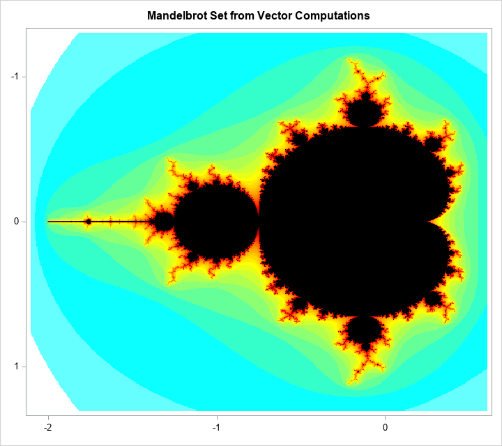
The last step is to assign colors that visualize the Mandelbrot set. Whereas Robert Allison used a scatter plot, I will use a heat map. The iters vector contains the number of iterations before divergence, or MaxIters if the trajectory never diverged. You can assign a color ramp to the number of iterations, or, as I've done below, to a log-transformation of the iteration number. I've previously discussed several ways to assign colors to a heat map.
/* Color parameter space by using LOG10(number of iterations) */ numIters = log10( shape(iters, nRe, nIm) ); /* shape iterations into matrix */ mandelbrot = numIters`; /* plot num iterations for each parameter */ call heatmapcont(mandelbrot) xValues=Re yValues=Im ColorRamp="Temperature" displayoutlines=0 showlegend=0 title="Mandelbrot Set from Vector Computations"; |
On my PC, the Mandelbrot computation takes about a second. This is not blazingly fast, but it is faster than the low-memory, non-vectorized, computation. If you care about the fastest speeds, use the DATA step, as shown in Robert's blog post.
I'm certainly not the first person to compute the Mandelbrot set, so what's the point of this exercise? The main purpose of this article is to show how to vectorize an iterative algorithm that performs the same computation many times for different parameter values. Rather than iterate over the set of parameter values and perform millions of scalar computations, you create an array (or matrix) of parameter values and perform a small number of vectorized computations. In most matrix-vector programming languages, a vectorized computation is more efficient than looping over each parameter value. There are few function calls and each call performs high-level computations on large matrices and vectors.
Statistical programmers don't usually have a need to compute fractals, but the ideas in this program apply to time series computations, root-finding, optimization, and any computation where you compute the same quantity for many parameter values. In short, although the Mandelbrot set is fun to compute, the ability to vectorize computations in a matrix language is a skill that rewards you with more than pretty pictures. And fast computations never go out of style.

2 Comments
Neat approach! (And I like the colors you chose for plotting your results!) :)
Pingback: How to draw a Mandelbrot set in SAS Visual Analytics - SAS Users