An analyst was using SAS to analyze some data from an experiment. He noticed that the response variable is always positive (such as volume, size, or weight), but his statistical model predicts some negative responses. He posted the data and asked if it is possible to modify the graph so that only positive responses are displayed.
This article shows how you can truncate a surface or a contour plot so that negative values are not displayed. You could do something similar to truncate unreasonably high values in a surface plot.
Why does the model predict negative values?
Before showing how to truncate the surface plot, let's figure out why the model predicts negative values when all the observed responses are positive. The following DATA step is a simplified version of the real data. The RSREG procedure uses least squares regression to fit a quadratic response surface. If you use the PLOTS=SURFACE option, the procedure automatically displays a contour plot and surface plot for the predicted response:
data Sample; input X Y Z @@; datalines; 10 90 22 22 76 13 22 75 7 24 78 14 24 76 10 25 63 5 26 62 10 26 94 20 26 63 15 27 94 16 27 95 14 29 66 7 30 69 8 30 74 8 ; ods graphics / width=400px height=400px ANTIALIASMAX=10000; proc rsreg data=Sample plots=surface(fill=pred overlaypairs); model Z = Y X; run; proc rsreg data=Sample plots=surface(3d fill=Pred gridsize=80); model Z = Y X; ods select Surface; ods output Surface=Surface; /* use ODS OUTPUT to save surface data to a data set */ run; |
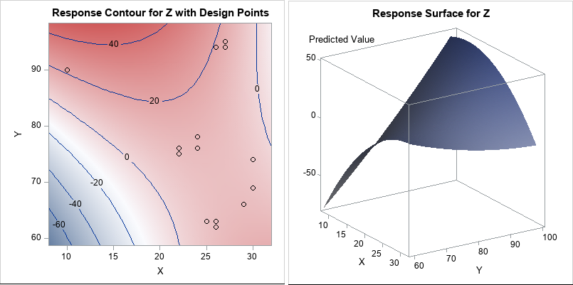
The contour plot overlays a scatter plot of the data. You can see that the data are observed only in the upper-right portion of the plot (the red regions) and that no data are in the lower-left portion of the plot. The RSREG procedure fits a quadratic model to the data. The predicted values near the observed data are all positive. Some of the predicted values that are far from the observed data are negative.
I previously wrote about this phenomenon and showed how to compute the convex hull for these bivariate data. When you evaluate the model inside the convex hull, you are interpolating. When you evaluate the model outside the convex hull, you are extrapolating. It is well known that polynomial regression models can give nonsensical results if you extrapolate far from the data.
Truncating a response surface
The RSREG procedure is not aware that the response variable should be positive. A quadratic surface will eventually get arbitrarily big in the positive and/or negative directions. You can see this on the contour and surface plots, which show the predictions of the model on a regular grid of (X, Y) values.
If you want to display only the positive portion of the prediction surface, you can replace each negative predicted value with a missing value. The first step is to obtain the predicted values on a regular grid. You can use the "missing value trick" to score the quadratic model on a grid, or you can use the ODS OUTPUT statement to obtain the gridded values that are used in the surface plot. I chose the latter option. In the previous section, I used the ODS OUTPUT statement to write the gridded predicted values for the surface plot to a SAS data set named Surface.
As Warren Kuhfeld points out in his article about processing ODS OUTPUT data set, the names in an ODS data object can be "long and hard to type." Therefore, I rename the variables. I also combine the gridded values with the original data so that I can optionally overlay the data and the predicted values.
/* rename vars and set negative responses to missing */ data Surf2; set Surface(rename=( Predicted0_1_0_0 = Pred /* rename the long ODS names */ Factor1_0_1_0_0 = GY /* 'G' for 'gridded' */ Factor2_0_1_0_0 = GX)) Sample(in=theData); /* combine with original data */ if theData then Type = "Data "; else Type = "Gridded"; if Pred < 0 then Pred = .; /* replace negative predictions with missing values */ label GX = 'X' GY = 'Y'; run; |
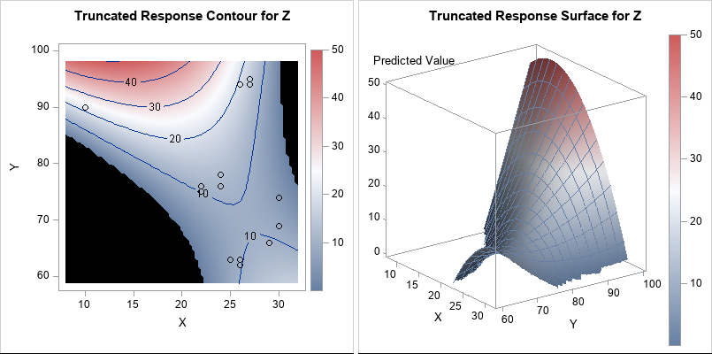
You can use the Graph Template Language (GTL) to generate graphs that are similar to those produced by PROC RSREG. You can then use PROC SGRENDER to create the graph. Because the negative response values were set to missing, the contour plot displays a missing value color (black, for this ODS style) in the lower-left and upper-right portions of the plot. Similarly, the missing values cause the surface plot to be truncated. By using the GRIDSIZE= option, you can make the jagged edges small.
Notice that the colors in the graphs are now based on the range [0, 50], whereas previously the colors were based on the range [-60, 50]. I've added a continuous legend to the plots so that the range of the response variable is obvious.
I'd like to stress that sometimes "nonsensical values" indicate an inappropriate model. If you notice nonsensical values, you should always ask yourself why the model is predicting those values. You shouldn't modify the prediction surface without a good reason. But if you do have a good reason, the techniques in this article should help you.
You can download the complete SAS program that analyzes the data and generates the truncated graphs.

2 Comments
I am not an IML user but ask that given the error below, does running the example file out of the package look like the polygon package install gives a folder under Packages with name polygon but the package itself expects the name is pol?
WARNING: Physical file does not exist, C:\Users\hans\OneDrive\Documents\My SAS Files\My SAS Files\IML\Packages\pol\source\PolyDrawImpl.iml.
ERROR: Cannot open %INCLUDE file C:\Users\hans\OneDrive\Documents\My SAS Files\My SAS Files\IML\Packages\pol/source/PolyDrawImpl.iml.
When polygon and identical pol folders both exist under Packages, no errors.
Instructions for installing packages are part of the SAS/IML documentation. You install the package by using the PACKAGE INSTALL statement in a PROC IML program. The zip file will be unzipped automatically into the directories under the 'polygon' folder.
The polygon package was used only to illustrate convex hulls. It is not needed for the statistical portion of the article, which is visualizing a truncated predicted surface. You can safely delete the three statements that use the polygon package.