Maybe if we think and wish and hope and pray
It might come true.
Oh, wouldn't it be nice?
The Beach Boys
Months ago, I wrote about how to use the EFFECT statement in SAS to perform regression with restricted cubic splines. This is the modern way to use splines in a regression analysis in SAS, and it replaces the need to use older macros such as Frank Harrell's %RCSPLINE macro. I shared my blog post with a colleague at SAS and mentioned that the process could be simplified. In order to specify the placement of the knots as suggested by Harrell (Regression Modeling Strategies, 2010 and 2015), I had to use PROC UNIVARIATE to get the percentiles of the explanatory variable. "Wouldn't it be nice," I said, "if the EFFECT statement could perform that computation automatically?"
I am happy to report that the 15.1 release of SAS/STAT (SAS 9.4M6) includes a new option that makes it easy to place internal knots at percentiles of the data.
You can now use the KNOTMETHOD=PERCENTILELIST option on the EFFECT statement to place knots. For example, the following statement places five internal knots at percentiles that are recommended in Harrell's book:
EFFECT spl = spline(x / knotmethod=percentilelist(5 27.5 50 72.5 95));
An example of using restricted cubic in regression in SAS
Restricted cubic splines are also called "natural cubic splines." This section shows how to perform a regression fit by using restricted cubic splines in SAS.
For the example, I use the same Sashelp.Cars data that I used in the previous article. For clarity, the following SAS DATA step renames the Weight and MPG_City variables to X and Y, respectively. If you want to graph the regression curve, you can sort the data by the X variable, but this step is not required to perform the regression.
/* create (X,Y) data from the Sashelp.Cars data. Sort by X for easy graphing. */ data Have; set sashelp.cars; rename mpg_city = Y weight = X model = ID; run; proc sort data=Have; by X; run; |
The following call to PROC GLMSELECT includes an EFFECT statement that generates a natural cubic spline basis using internal knots placed at specified percentiles of the data. The MODEL statement fits the regression model and the OUTPUT statement writes an output data set that contains the predicted values. The SGPLOT procedure displays a graph of the regression curve overlaid on the data:
/* fit data by using restricted cubic splines using SAS/STAT 15.1 (SAS 9.4M6) */ ods select ANOVA ParameterEstimates SplineKnots; proc glmselect data=Have; effect spl = spline(X/ details naturalcubic basis=tpf(noint) knotmethod=percentilelist(5 27.5 50 72.5 95) ); /* new in SAS/STAT 15.1 (SAS 9.4M6) */ model Y = spl / selection=none; /* fit model by using spline effects */ output out=SplineOut predicted=Fit; /* output predicted values */ quit; title "Restricted Cubic Spline Regression"; title2 "Five Knots Placed at Percentiles"; proc sgplot data=SplineOut noautolegend; scatter x=X y=Y; series x=X y=Fit / lineattrs=(thickness=3 color=red); run; |
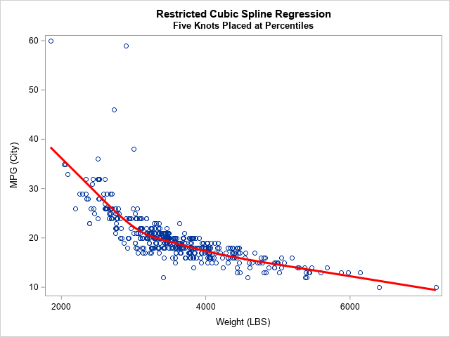
In summary, the new KNOTMETHOD=PERCENTILELIST option on the EFFECT statement simplifies the process of using percentiles of a variable to place internal knots for a spline basis. The example shows knots placed at the 5th, 27.5th, 50th, 72.5th, and 95th percentiles of an explanatory variable. These heuristic values are recommended in Harrell's book. For more details about the EFFECT statement and how the location of knots affects the regression fit, see my previous article "Regression with restricted cubic splines in SAS."
You can download the complete SAS program that generates this example, which requires SAS/STAT 15.1 (SAS 9.4M6). If you have an earlier release of SAS, the program also shows how to perform the same computations by calling PROC UNIVARIATE to obtain the location of the knots.

28 Comments
Thank you for your wonderful work. And I want to konw how to adjusted other confounders in the restricted cubic spline.
Hi,
I have 4 knots.
Is there anyway to get the parameters for the curve between the second and third knots, third and fourth knots, etc.
Thank you.
Yes. When you use knots in a linear regression, you will get estimates for the regression coefficients. The curve of the predicted values is therefore a linear combination of the spline basis, as shown in the article "Visualize a regression with splines." If you want to restrict the interval between the second and third knots, just add together the knots with nonzero support on that interval.
can we add spline model in proc MCMC ?
You can use spline effects in any SAS procedure.
1. Use the OUTDESIGN= option in PROC GLMSELECT to output the spline basis to a data set, as shown in the articles
"Regression with restricted cubic splines in SAS"
and
"Visualize a regression with splines"
2. Use the spline bases as explanatory variables in the model.
Thank you for your wonderful work. And I want to konw how to adjusted other confounders in the restricted cubic spline.
You can add other effects on the MODEL statement. If you have specific data or syntax that you want to discuss, you can post them to the SAS Support Communities.
Hi Rick,
I have 9 data points and I would like to ask you if it's appropriate to apply regression with restricted cubic splines. I have the scatterplot from sgplot, but I can't add it here. The plot shows an upward quadratic then decreases linearly. I will be happy to send the display.
Thanks!
Sure. Go ahead.
This forum doesn't support tables or graphs. I don't have your email. How can I share it with you?
Sorry that I was unclear. I meant "Sure, go ahead and fit a cubic spline model to 9 data points."
If you need more help, you can post questions to the SAS Support Communities. The Communities enable you to upload data, programs, and graphics.
Hi Rick,
Thank you for this post and your comments. They are really helpful.
Following your above SAS syntax, I wrote the following one (Model one), by specifying the values at each knot.
I then created 3 spline variables and wrote model two. The results generated by the two models are almost the same, except the coefficients of the thee spline variables (the t-values and p-values are the same. Would you please share with me your thoughts about the differences?
Many thanks, Hongjie
Your definitions of the spline variables (term2-term4) are wrong. You do not need to use a separate DATA step to generate the spline effects because PROC GLMSELECT will give them to you. See the article, "Visualize a regression with splines."
If you add OUTDESIGN=Splines option to the PROC GLMSELECT statement, then you can reproduce the parameter estimates by using the following:
Hi Rick,
Thank you very much for your quick help!
Do you happen to know how the SAS EFFECT statement calculates SPLs for each subject or what equation it uses? I could not find references from SAS.
As mentioned in "Regression with restricted cubic splines in SAS," the EFFECT statement uses the definition from The Elements of Statistical Learning (Hastie, Tibshirani, and Friedman, 2009, 2nd Ed, pp. 144-146).
Great and thanks! Hongjie
Hi Rick,
I have to manually create basis functions for a variable but SAS doesn't seem to have a procedure to do it. I am using Frank Harrell's macro RCSPLINE but the basis variables are not identical to those created by SAS using OUTDESIGN. It seems like SAS is dividing the second basis by 4 and the last one by 4.5. Not sure where these numbers come from for the example given below. Why are SAS numbers different from the ones created by the macro?
data simulation;
do i=1 to 10000;
t=rand('uniform',0,10);
p=1/(1+exp(sin(t)));
y=rand('bernoulli',p);
output;
end;
run;
*model a natural cubic spline;
*and store the result in "mystore";
proc logistic data=simulation OUTDESIGN=splines;
effect myspline=spline(t/knotmethod=list(1,2,3,4) NATURALCUBIC);
model y(event="1")=myspline;
store mystore;
run;
/*-------------------------
MACRO FOR CUBIC SPLINES
-------------------------*/
%macro rcspline(x,knot1,knot2,knot3,knot4,knot5,knot6,knot7,knot8,knot9,knot10, norm=2);
%LOCAL j v7 k tk tk1 t k1 k2;
%LET v7=&x; %IF %length(&v7)=8 %THEN %LET v7=%SUBSTR(&v7,1,7);
%*get no. knots, last knot, next to last knot;
%DO k=1 %TO 10;
%IF %QUOTE(&&knot&k)= %THEN %GOTO nomorek;
%END;
%LET k=11;
%nomorek: %LET k=%EVAL(&k-1); %LET k1=%EVAL(&k-1); %LET k2=%EVAL(&k-2);
%IF &k<3 %THEN %PUT ERROR: <3 knots given. no spline variables CREATEd.;
%ELSE %DO;
%LET tk=&&knot&k;
%LET tk1=&&knot&k1;
DROP _kd_; _kd_=
%IF &norm=0 %THEN 1;
%ELSE %IF &norm=1 %THEN &tk - &tk1;
%ELSE (&tk - &knot1)**.666666666666; ;
%DO j=1 %TO &k2;
%LET t=&&knot&j;
&v7&j=max((&x-&t)/_kd_,0)**3+((&tk1-&t)*max((&x-&tk)/_kd_,0)**3
-(&tk-&t)*max((&x-&tk1)/_kd_,0)**3)/(&tk-&tk1)%STR(;);
%END;
%END;
%mend rcspline;
**comparing to splines datasets from PROC LOGISTIC
**t1 from PROC LOGISTIC=t1 from below divided by 4-1=3;
DATA want; SET simulation;
%rcspline(t,1,2,3,4);
RUN;
Near the end of my previous article about splines, I explain why the basis functions are not equal, but the predicted values are the same. Briefly, the macro uses a different scaling.
Thank you Rick!
I am also looking to implement penalized spline and I was wondering if there is a way to do so in SAS. I am looking for a SAS equivalent of the R- PSPLINE functionthat can be used in PROC LOGISTIC.
I don't know what the R function does, but Harrell has a %PSLINE macro for SAS. For a discussion and example, see https://www.lexjansen.com/sesug/2019/SESUG2019_Paper-233_Final_PDF.pdf or Harrell's site http://biostat.mc.vanderbilt.edu/wiki/pub/Main/SasMacros/survrisk.txt
Harells %PSLINE macro is for plotting the restricted cubic spline. The PSPLINE function is R is a piecewise polynomial with a smoothing penalty. I am not sure if SAS has anything at the moment.
I just found out that there is a PSPLINE(x) that can be used only in PROC TRANSREG. I am running conditional logit so I cannot use it in PROC LOGISTIC or PROC PHREG.
Hi Rick,
Will this approach work with PROC PHREG?
Yes. PROC PHREG supports the EFFECT statement, so you can create spline effects and use them as explanatory variables in the P-H model.
Hello Rick,
I am having trouble creating these visualizations in SAS using PROC PHREG. I tried using your code above by trying to request an output dataset with predicted fit values using the following line within PHREG: OUTPUT out =SplineOut predicted = Fit;. However, it does not seem as if PHREG supports requesting predicted fit. Is there some other way to get a similar graph in PHREG? Thanks.
Check the doc. The SURVIVAL= keyword on the OUTPUT statement enables you to output a variable that contains the survival probability.
Hi Rick,
I would like to ask you if you have used the %RCS_reg package, I am using it and I have found that I can run the results but I cannot generate the RCS curves. The log reports an error saying, I would like to consult you on what this can be done. Here is my code%RCS_Reg( infile= NHSALL_2, outfile= NHSALL_out,
Dir_data= ,
Main_spline_var= LBXVIDMS, ref_val= , AVK_msv= 0, knots_msv=5 50 95,
Oth_spline_var1=,
typ_reg= cox,
dep_var= mort_all, surv_time_var= PERyear_EXM,
adjust_var=sex1 sex2 race1 race2 race3 race4 BMI1 BMI2 BMI2 edu1
edu2 edu3 income1 income2 income3 drinking1 drinking2
drinking3 smoking1 smoking2 smoking3 phyacty1 phyacty2 phyacty3
DURDM1 DURDM2 DURDM3 MEDDM1 MEDDM2 MEDDM3 MEDDM4
hbp cvd ghpgp hbc,
Y_ref_line= 1, max_Xaxis= ,
exp_beta= 1, round=,
specif_val= );
quit;
. The variables are converted to dummy variables except for age which is continuous.
No, I have never used that macro. Now that SAS regression routines support spline effects natively, there is no need to run a third-party macro from 2008.