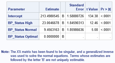
I remember the first time I used PROC GLM in SAS to include a classification effect in a regression model. I thought I had done something wrong because the parameter estimates table was followed by a scary-looking note:
Note: The X'X matrix has been found to be singular, and a generalized inverse
      was used to solve the normal equations. Terms whose estimates are
      followed by the letter 'B' are not uniquely estimable.
Singular matrix? Generalized inverse? Estimates not unique? "What's going on?" I thought.
In spite of the ominous note, nothing is wrong. The note merely tells you that the GLM procedure has computed one particular estimate; other valid estimates also exist. This article explains what the note means in terms of the matrix computations that are used to estimate the parameters in a linear regression model.
The GLM parameterization is a singular parameterization
The note is caused by the fact that the GLM model includes a classification variable. Recall that a classification variable in a regression model is a categorical variable whose levels are used as explanatory variables. Examples of classification variables (called CLASS variables in SAS) are gender, race, and treatment. The levels of the categorical variable are encoded in the columns of a design matrix. The columns are often called dummy variables. The design matrix is used to form the "normal equations" for least squares regression. In terms of matrices, the normal equations are written as (X`*X)*b = X`*Y, where X is a design matrix, Y is the vector of observed responses, and b is the vector of parameter estimates, which must be computed.
There are many ways to construct a design matrix from classification variables. If X is a design matrix that has linearly dependent columns, the crossproduct matrix X`X is singular. Some ways of creating the design matrix always result in linearly dependent columns; these constructions are said to use a singular parameterization.
The simplest and most common parameterization encodes each level of a categorical variable by using a binary indicator column. This is known as the GLM parameterization. It is a singular parameterization because if X1, X2, ..., Xk are the binary columns that indicate the k levels, then Σ Xi = 1 for each observation.
Not surprisingly, the GLM procedure in SAS uses the GLM parameterization. Here is an example that generates the "scary" note. The data are a subset of the Sashelp.Heart data set. The levels of the BP_Status variable are "Optimal", "Normal", and "High":
data Patients; set Sashelp.Heart; keep BP_Status Cholesterol; if ^cmiss(BP_Status, Cholesterol); /* discard any missing values */ run; proc glm data=Patients plots=none; class BP_Status; model Cholesterol = BP_Status / solution; quit; |
If you change the reference levels, you get a different estimate
If you have linearly dependent columns among the explanatory variables, the parameter estimates are not unique. The easiest way to see this is to change the reference level for a classification variable. In PROC GLM, you can use the REF=FIRST or REF=LAST option on the CLASS statement to change the reference level. However, the following example uses PROC GLMSELECT (without variable selection) because you can simultaneously use the OUTDESIGN= option to write the design matrix to a SAS data set. The first call writes the design matrix that PROC GLM uses (internally) for the default reference levels. The second call writes the design matrix for an alternate reference level:
/* GLMSELECT can fit the data and output a design matrix in one step */ title "Estimates for GLM Paremeterization"; title2 "Default (Last) Reference Levels"; ods select ParameterEstimates(persist); proc glmselect data=Patients outdesign(fullmodel)=GLMDesign1; class BP_Status; model Cholesterol = BP_Status / selection=none; quit; /* Change reference levels. Different reference levels result in different estimates. */ title2 "Custom Reference Levels"; proc glmselect data=Patients outdesign(fullmodel)=GLMDesign2; class BP_Status(ref='Normal'); model Cholesterol = BP_Status / selection=none; quit; ods select all; /* compare a few rows of the design matrices */ proc print data=GLMDesign1(obs=10 drop=Cholesterol); run; proc print data=GLMDesign2(obs=10 drop=Cholesterol); run; |
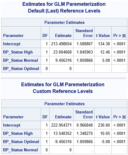
The output shows that changing the reference level results in different parameter estimates. (However, the predicted values are identical for the two estimates.) If you use PROC PRINT to display the first few observations in each design matrix, you can see that the matrices are the same except for the order of two columns. Thus, if you have linearly dependent columns, the GLM estimates might depend on the order of the columns.
The SWEEP operator produces a generalized inverse that is not unique
You might wonder why the parameter estimates change when you change reference levels (or, equivalently, change the order of the columns in the design matrix). The mathematical answer is that there is a whole family of solutions that satisfy the (singular) regression equations, and from among the infinitely many solutions, the GLM procedure chooses the solution for which the estimate of the reference level is exactly zero.
Last week I discussed generalized inverses, including the SWEEP operator and the Moore-Penrose inverse. The SWEEP operator is used by PROC GLM to obtain the parameter estimates. The SWEEP operator produces a generalized inverse that is not unique. In particular, the SWEEP operator computes a generalized inverse that depends on the order of the columns in the design matrix.
The following SAS/IML statements read in the design matrices for each GLM parameterization and use the SWEEP function to reproduce the parameter estimates that are computed by the GLM procedure. For each design matrix, the program computes solutions to the normal equations (X`*X)*b = (X`*Y). The program also computes the Moore-Penrose solution for each design matrix.
proc iml; /* read design matrix and form X`X and X`*Y */ use GLMDesign1; read all var _NUM_ into Z[c=varNames]; close; p = ncol(Z); X = Z[, 1:(p-1)]; Y = Z[, p]; vNames = varNames[,1:(p-1)]; A = X`*X; c = X`*Y; /* obtain G2 and Moore-Penrose solution for this design matrix */ Sweep1 = sweep(A)*c; GInv1 = ginv(A)*c; print Sweep1[r=vNames], GInv1; /* read other design matrix and form X`X and X`*Y */ use GLMDesign2; read all var _NUM_ into Z[c=varNames]; close; p = ncol(Z); X = Z[, 1:(p-1)]; Y = Z[, p]; vNames = varNames[,1:(p-1)]; A = X`*X; c = X`*Y; /* obtain G2 and Moore-Penrose solution for this design matrix */ Sweep2 = sweep(A)*c; GInv2 = ginv(A)*c; print Sweep2[r=vNames], GInv2; |
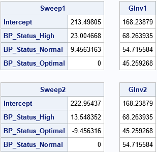
The results demonstrate that the SWEEP solution depends on the order of columns in a linearly dependent design matrix. However, the Moore-Penrose solution does not depend on the order. The Moore-Penrose solution is the same no matter which reference levels you choose for the GLM parameterization of classification effects.
Some estimates are unique
It is worth mentioning that although the parameter estimates are not unique, there are other statistics that are unique and that do not depend on the order in which the crossproduct matrix is swept or the reference level. An example is a difference between the means of two class levels. The SAS/STAT documentation contains a chapter that discusses these so-called estimable functions.
Summary
In summary, the scary note that PROC GLM produces reminds you of the following mathematical facts:
- When you include classification effects in a linear regression model and use the GLM parameterization to construct the design matrix, the design matrix has linearly dependent columns.
- The X`X matrix is singular when X has linearly dependent columns. Consequently, the parameter estimates for least squares regression are not unique.
- From among the infinitely many solutions to the normal equations, the solution that PROC GLM (and other SAS procedures) computes is based on a generalized inverse that is computed by using the SWEEP operator.
- The solution obtained by the SWEEP operator depends on the reference levels for the CLASS variables.
If the last fact bothers you (it shouldn't), an alternative estimate is available by using the GINV function to compute the Moore-Penrose inverse. The corresponding estimate is unique and does not depend on the reference level.

11 Comments
Stated a bit more explicitly, PROC GLM does a sequential sweep. That is, it sweeps (enters into the model) the first term or pivot (the intercept), then the second term, and so on. When it hits the last level of a categorical variable, then it can't sweep that pivot because that column is a linear combination of preceding columns. This behavior goes back to the earliest days of GLM. Software could instead choose to sweep the pivots in a different order. Then you would get different results. We have a subroutine at SAS--one I initially wrote--that does nonsequential sweeps. Instead, it finds the best pivot to sweep on each time from the pivots that have not yet been swept. The TRANSREG procedure uses this method, it sweeps with rational pivoting, rather than performing sequential sweeps. This can lead to more accurate results, particularly for problems that are contrived to be numerically difficult. The SWEEPR (r for rational pivoting) function gets called in dozens of other places throughout SAS. GLM does not use it because it needs to compute Type I sums of squares, which are based on sequential sweeps. When I wrote TRANSREG, my goals were different from GLM's goals, so I did things differently. In particular, I wanted to give the user complete control over the coding and choice of reference levels and default to a full-rank coding rather than rely on a less-than-full rank coding.
Thank you Rick for another very good article, again superbly written thus making it easy to follow along (and learn!!). Every now and then I may get confused on a given SAS author's point, but never (knock on wood) has this occurred when reading your work.
Pingback: 4 ways to compute an SSCP matrix - The DO Loop
This is a very helpful article. I do have one question regarding this statement in the article: "It is worth mentioning that although the parameter estimates are not unique, there are other statistics that are unique and that do not depend on the order in which the crossproduct matrix is swept or the reference level. An example is a difference between the means of two class levels."
How does the fact that the estimate for a categorical is not unique affect the interpretation of the Pvalue for that predictor? Will the p-value interpretation always be significant or non significant for that predictor even if the estimate changes?
I assume you are talking about the p-value for the estimates of the individual levels of the class variable? They depend on the parameterization and are not unique. In general, if you can do something that changes the value of a statistic (e.g., change the parameterization or the order of the variables in the model), then hypothesis tests that use that statistic will also change.
Hi Rick, I'd like to know how to reduce columns that are linear combinations of others and make the crossproduct of design matrix non-singular.
I am think of using the following method:
Suppose x is the design matrix:
call qr(q, r, piv, lindep, x);
x = x[, piv[1: lindep]];
You can choose a model without an intercept to avoid linear dependency between columns.
Yes, if you have a model with only one CLASS variable. With one CLASS variable, the intercept gets "transferred" to the reference level of the CLASS variable. However, if you have two or more CLASS variables, fitting a NOINT model does not eliminate the warning.
Indeed, so except for 1-way model it seems no way around to make all columns of the design matrix linearly independent.
No, that's not correct. Yes, the GLM parameterization is a singular parameterization. However, as the article mentions, there are other parameterizations that result in design matrices with independent columns. See the link in the article for more information.
If you have SAS programming questions, I encourage you to post them to the SAS Support Communities.
Nice to know. Thanks! Maybe I should say only for one-way classification model, there exists a both intuitive (simple) and linear independent parameterization?
One-way model seems unique in some ways. Another example is that its least square means are the same as arithmetic group means for unbalanced design which does not hold for multi-class models. I can find ambiguous wording that may have ignored/forgot this special case (one-way) in web posting, for example, https://online.stat.psu.edu/stat502_fa21/lesson/3/3.5.
"Note also that the least square means are the same as the original arithmetic means that were generated in the Summary procedure in Section 3.3 because all 4 groups have the same sample sizes. With unequal sample sizes or if there is a covariate present, the least square means can differ from the original sample means."