Will the real Pareto distribution please stand up?
SAS supports three different distributions that are named "Pareto." The Wikipedia page for the Pareto distribution lists five different "Pareto" distributions, including the three that SAS supports. This article shows how to fit the two-parameter Pareto distribution in SAS and discusses the relationship between the "standard" Pareto distribution and other "generalized" Pareto distributions.
The Pareto distribution
To most people, the Pareto distribution refers to a two-parameter continuous probability distribution that is used to describe the distribution of certain quantities such as wealth and other resources. This "standard" Pareto is sometimes called the "Type I" Pareto distribution.
The SAS language supports the four essential functions for working with the Type I Pareto probability distribution (PDF, CDF, quantiles, and random number generation).
The Pareto density function is usually written as
f(x) = α xmα / xα + 1
where the shape parameter α > 0 describes how quickly the density decays and the scale parameter xm > 0 is the minimum possible value of x. The Roman letter a is sometimes used in place of the Greek letter α.
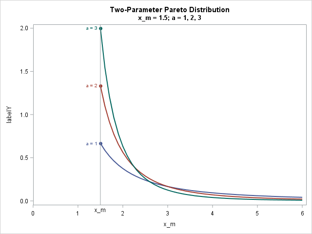
The following graph shows three density curves for xm = 1.5 and for three values of a (or α):
Fit the Pareto distribution in SAS
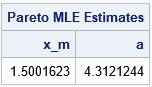
There are two ways to fit the standard two-parameter Pareto distribution in SAS. It turns out that the maximum likelihood estimates (MLE) can be written explicitly in terms of the data. Therefore, you can use SAS/IML (or use PROC SQL and the DATA step) to explicitly compute the estimates, as shown below:
/* MLE estimate for standard two-parameter Pareto. For the formula, see https://en.wikipedia.org/wiki/Pareto_distribution#Parameter_estimation */ proc iml; use Pareto; read all var "x"; close; x_m = min(x); /* MLE estimate of scale param */ a = countn(x) / sum(log(x/x_m)); /* MLE estimate of shape param */ Est = x_m || a; print Est[c={"x_m" "a"} L="Pareto MLE Estimates"]; quit; |
The second way to fit the Pareto distribution is to use PROC NLMIXED, which can fit general MLE problems. You need to be a little careful when estimating the x_m parameter because that parameter must be less than or equal to the minimum value in the data. In the following, I've used a macro variable that contains the minimum value of the data to constrain the MLE estimates to be in the interval (0, min(x)]:
proc sql; select Min(x) into :minX from Pareto; /* store x_m in macro */ run; proc nlmixed data=Pareto; parms x_m 1 a 2; * initial values of parameters; bounds 0 < x_m < &minX, a > 0; * bounds on parameters; LL = log(a) + a*log(x_m) - (a+1)*log(x); * or use logpdf("Pareto", x, a, x_m); model x ~ general(LL); run; |
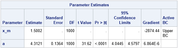
Notice that the MLE estimates optimize the constrained log-likelihood (LL) function, but the gradient does not vanish at the optimal parameter values. This explains why the output from PROC NLMIXED does not include an estimate for the standard error or confidence intervals for the x_m parameter. You do, however, get an estimate for the standard error of the shape parameter, which is not available from the direct computation of the point estimate.
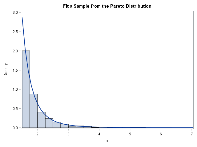
If you overlay a histogram and the density estimate for the fitted parameters, you obtain the following graph, which shows that the Pareto curve fits the data well.
Pareto versus generalized Pareto distributions
The previous section shows how to fit the two-parameter (Type I) Pareto distribution in SAS. Unfortunately, some SAS programmers see that PROC UNIVARIATE supports a PARETO option on the HISTOGRAM statement, and assume that it is the usual two-parameter Pareto distribution. It is not. The UNIVARIATE procedure supports a generalized Pareto distribution, which is different from the standard distribution.
The UNIVARIATE procedure fits a generalized (Type II) Pareto distribution, which has three parameters: the threshold parameter θ, the scale parameter σ, and a shape parameter. Unfortunately, the UNIVARIATE documentation refers to the shape parameter as α, but it is not the same parameter as in the standard two-parameter Pareto distribution. In particular, the shape parameter in PROC UNIVARIATE can be positive or negative. The three-parameter generalized (Type II) Pareto distribution reduces to the standard Pareto when θ = -σ / α. Call that common value xm and define β = -1 / α. Then you can show that the PDF of the generalized Pareto (as supported in PROC UNIVARIATE) reduces to the standard Type I Pareto (which is supported by the PDF, CDF, and RAND functions). In general, however, the three-parameter generalized Pareto distribution can fit a wider variety of density curves than the two-parameter Pareto can.
The UNIVARIATE parameterization is similar to the parameterization for the Type II generalized Pareto distribution that is listed in the Wikipedia article. If you start with the UNIVARIATE parameterization and define s = -σ / α and β = -1 / α, then you obtain the parameterization in the Wikipedia article.
You can use PROC NLMIXED to fit any of the generalized Pareto distributions. I've already shown how to fit the Type I distribution. Two other procedures in SAS support other generalized Pareto distributions:
- You can fit the Type II distribution by using PROC UNIVARIATE.
- You can fit the Lomax distribution by using PROC SEVERITY in SAS/ETS software.
It is a real annoyance to have so many different versions of the Pareto distribution, but such is life. With apologies to the Gershwin brothers, I'll end with a reference to the old song, "Let's Call the Whole Thing Off":
You say Pareto, and I say Par-ah-to.
Pareto, Par-ah-to, generalized Pareto?
Let's call the whole thing off!
If you don't want to "call the whole thing off," hopefully this article explains the different forms of the Pareto distributions in SAS and how to estimate the parameters in these models.
