Every day I’m shufflin'.
Shufflin', shufflin'.
-- "Party Rock Anthem," LMFAO
The most popular way to mix a deck of cards is the riffle shuffle, which separates the deck into two pieces and interleaves the cards from each piece. Besides being popular with card players, the riffle shuffle is well-known among statisticians because Bayer and Diaconis (1992) showed that it takes seven riffle shuffles to randomize a 52-card deck. This result annoyed many recreational card players because shuffling seven times "slows down the game".
The second most popular shuffling technique is the overhand shuffle. The overhand shuffle is much less efficient at mixing the cards than a riffle shuffle. A result by Pemantle (1989) indicates that at least 50 overhand shuffles are required to adequately mix the deck, but computer experiments (Pemantle, 1989, p. 49) indicate that in many situations 1,000 or more overhand shuffles are required to randomize a deck. Talk about slowing down the game! This article shows how to simulate an overhand shuffle in SAS and visually compares the mixing properties of the riffle and overhand shuffles.
The overhand shuffle
An overhand shuffle transfers a few cards at a time from the dealer's right hand to his left. The dealer slides a few cards from the top of the deck in his right hand into his left hand. The process is repeated until all cards in his right hand are transferred. Consequently, cards that started near the top of the deck end up near the bottom, and vice versa.
Mathematically, you can model an overhand shuffle by randomly choosing k cut points that separate the deck into k+1 "packets" of contiguous cards. The size of a packet can vary, as can the number of packets. The overhand shuffle reverses the order of the packets while preserving the order of the cards within each packet. When the packet sizes are small, the cards are mixed better than when the packets are bigger.
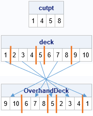
For example, a deck that contains 10 cards (enumerated 1-10) might be split into five packets such as (1)(234)(5)(678)(9 10), where the parentheses show the cards in each of the packets. In this example, the cut points are the locations after cards 1, 4, 5, and 8. The packets contain 1, 3, 1, 3, and 2 cards. The overhand shuffle reverses the order of the packets, so the deck is reordered as (9 10)(678)(5)(234)(1). This is shown in the following graphic.
In a statistical model of the overhand shuffle, the cut points are assumed to be randomly chosen with probability p from among the N-1 possible locations between adjacent cards. An ideal overhand shuffle uses p = 1/2, which results in packets that are typically sized, 1, 2, and 3 (the packet size is geometrically distributed). However, among amateurs, the probability is much lower and an overhand shuffle reorders only a few large packets, which can lead to poor mixing of the cards.
Simulate an overhand shuffle
I previously showed how to simulate a riffle shuffle in the SAS/IML language. The following program shows how to simulate an overhand shuffle. The deck of cards (represented as a vector of integers with the values 1 to N) is passed in, as is the probability of choosing a cut point. To test the program, I pass in a deck that has 10 cards enumerated by the integers 1–10. The new order of the deck was shown in the previous section.
proc iml; call randseed(1234); /* Simulate overhand shuffle. Randomly split deck into k packets. Reverse the order of the packets. Each position between cards is chosen to be a cut point with probability p. (Default: p=0.5) */ start Overhand(_deck, p=0.5); deck = colvec(_deck); /* make sure input is column vector */ N = nrow(deck); /* number of cards in deck */ b = randfun(N-1, "Bernoulli", p); /* randomly choose cut points */ if all(b=0) then return _deck; /* no cut points were chosen */ cutpt = loc(b=1); /* cut points in range 1:n-1 */ cutpt = 0 || cutpt || N; /* append 0 and n */ rev = n - cutpt + 1; /* reversed positions */ newDeck = j(N, 1, .); do i = 1 to ncol(cutpt)-1; /* for each packet... */ R = (1 + cutpt[i]):cutpt[i+1]; /* positions of cards in right hand */ L = rev[i+1]:(rev[i]-1); /* new positions in left hand */ newDeck[L] = deck[R]; /* transfer packet from right to left hand */ end; return shape(newDeck, nrow(_deck), ncol(_deck)); /* return same shape as input */ finish; deck = 1:10; OverhandDeck = Overhand(deck, 0.5); print deck; print OverhandDeck; |
Simulate many overhand shuffles
Let's now consider the standard 52-card deck, represented by the integers 1–52. The following loop performs 10 overhand shuffles (p = 0.5) and uses a heat map to show the order of the cards after each shuffle:
N = 52; /* standard 52-card deck */ deck = 1:N; /* initial order */ numShuffles = 10; /* number of times to shuffle cards */ OverDeck = j(numShuffles+1, N); OverDeck[1,] = deck; do i = 2 to numShuffles + 1; OverDeck[i,] = Overhand(OverDeck[i-1,]); end; ramp = palette("YLORBR",9); call heatmapcont(OverDeck) colorramp=ramp yvalues=0:numShuffles title="Positions of 52 Cards After Overhand Shuffles"; |
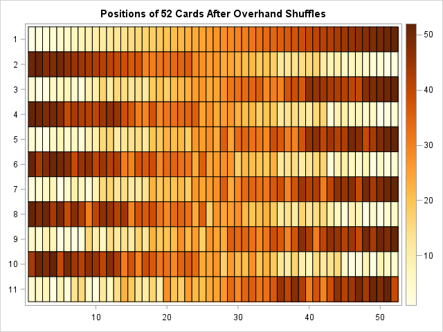
The cell colors in the heat map correspond to the initial position of the cards: light colors indicate cards that are initially near the top of the deck and dark colors represent cards that are initially near the bottom of the deck. The first row shows the initial positions of the cards in the deck. The second row shows the cards after one overhand shuffle. The third row shows the cards after two overhand shuffles, and so on. It is interesting to see how the pattern changes if you use p=0.25 or p=0.1. Try it!
One feature that is apparent in the image is that the relative positions of cards depend on whether you have performed an even or an odd number of overhand shuffles. After an odd number of shuffles, the top of the deck contains many cards that were initially at the bottom, and the bottom of the deck contains cards that were initially at the top. After an even number of shuffles, the top of the deck contains many cards that were initially at the top. Another apparent feature is that this process does not mix the cards very well. The last row in the heat map indicates that after 10 overhand shuffles, many cards are not very far from their initial positions. Furthermore, many cards that were initially next to each other are still within a few positions of each other.
Maybe additional overhand shuffles will address these deficiencies? The following program simulates 100 overhand shuffles. To aid in the visualization, the heat map shows only the results after 2, 4, 6, ..., and 100 shuffles (the even numbers):
deck = 1:N; /* reset initial order */ numShuffles = 100; /* number of times to shuffle cards */ numEvenShuffles = numShuffles / 2; OverDeck = j(numEvenShuffles+1, N); OverDeck[1,] = deck; /* save only the EVEN shuffles */ do i = 2 to numEvenShuffles + 1; OverDeck[i,] = Overhand(Overhand( OverDeck[i-1,] )); /* 2 calls */ end; call heatmapcont(OverDeck) colorramp=ramp yvalues=0:numEvenShuffles title="Positions of 52 Cards After EVEN Overhand Shuffles"; |
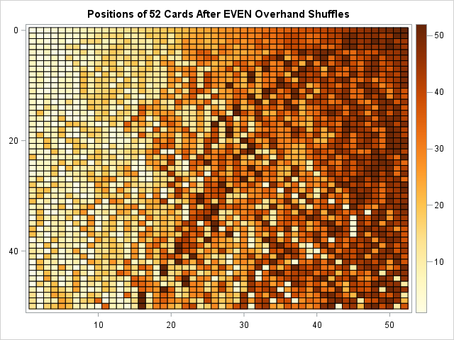
The heat map indicates that the deck is not well-mixed even after 100 overhand shuffles. Look at the last row in the heat map, which shows the positions of the cards in the deck colored by their initial position. There are a small number of light-colored cells on the right side of the heat map (cards that were initially on top; now near the bottom), and a small number of dark-colored cells on the left side of the heat map (cards that were initially on the bottom; now near the top). However, in general, the left side of the heat map contains mostly light-colored cells and the right side contains mostly dark-colored cells, which indicates that cards that have not moved far from their initial positions.
If you use smaller values of p (that is, the average packet size is larger), you will observe different patterns. The theory says that large packets cause nearby cards to tend to stay together for many shuffles. Jonasson (2006) was able to prove that if a deck has N cards, then O(N2 log(N)) overhand shuffles are required to randomize the deck. This compares with (3/2) log2(N) for the riffle shuffle, which is presented in the next section.
A comparison with the riffle shuffle
The riffle shuffle, which randomizes a deck after about seven shuffles. You can simulate a riffle shuffle in SAS and create a similar heat map. The following heat map shows the order of a 52-card deck after each of 10 riffle shuffles:
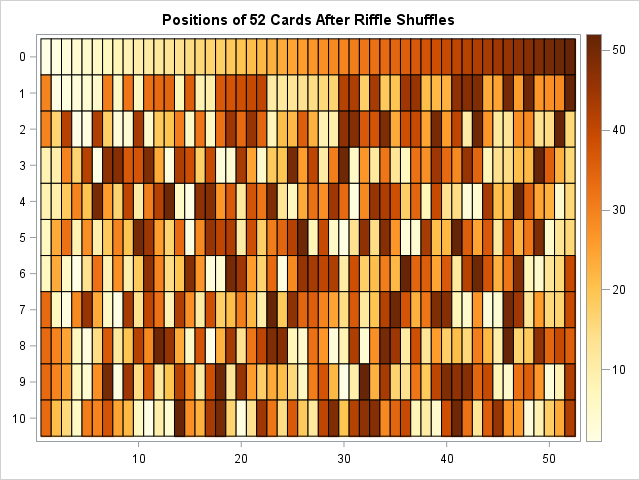
The heat map shows how quickly a riffle shuffle randomizes a deck. The last row (after 10 riffles) shows that light-colored cells are distributed throughout the deck, as are dark-colored cells and medium-colored cells. Furthermore, this behavior seems to occur after six or seven rows (at least to my untrained eye). I cannot see much difference between the "randomness" in row 6 and row 10. However, theoretically, a card in an earlier row (say, row 5) is more likely to be near cards that were initially close to it. For example, a dark-colored cell in row 5 is more likely to be near another dark-colored cell than would be expected in a randomized deck. However, by the time you perform 7 or more riffle shuffles, two cards that started near each other might be located far apart or might be close to each other. You cannot predict which will occur because the cards have been randomized.
In summary, the overhand shuffle does not mix cards very well. The simulation indicates that an overhand shuffle is not effective at separating cards that begin near each other. Even after 100 overhand shuffles (with p=0.5), the positions of many cards are only slightly different from their initial positions. In contrast, a riffle shuffle is an effective way to randomize a deck in approximately seven shuffles.

1 Comment
Hi Rick - Very interesting. How many shuffles would it take to randomize if you did a combination of overhand method and rifle method? Would the order matter - for example,.alternating rifle and overhand versus rifle first followed by overhand. Would the overhand method have any impact?