A SAS programmer recently asked how to interpret the "standardized regression coefficients" as computed by the STB option on the MODEL statement in PROC REG and other SAS regression procedures. The SAS documentation for the STB option states, "a standardized regression coefficient is computed by dividing a parameter estimate by the ratio of the sample standard deviation of the dependent variable to the sample standard deviation of the regressor." Although correct, this definition does not provide an intuitive feeling for how to interpret the standardized regression estimates. This article uses SAS to demonstrate how parameter estimates for the original variables are related to parameter estimates for standardized variables. It also derives how regression coefficients change after a linear transformation of the variables.
Proof by example
One of my college physics professors used to smile and say "I will now prove this by example" when he wanted to demonstrate a fact without proving it mathematically. This section uses PROC STDIZE and PROC REG to "prove by example" that the standardized regression estimates for data are equal to the estimates that you obtain by standardizing the data. The following example uses continuous response and explanatory variables, but there is a SAS Usage Note that describes how to standardize classification variables.
The following call to PROC REG uses the STB option to compute the standardized parameter estimates for a model that predicts the weights of 19 students from heights and ages:
proc reg data=Sashelp.Class plots=none; Orig: model Weight = Height Age / stb; ods select ParameterEstimates; quit; |
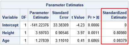
The last column is the result of the STB option on the MODEL statement. You can get the same numbers by first standardizing the data and then performing a regression on the standardized variables, as follows:
/* Put original and standardized variables into the output data set. Standardized variables have the names 'StdX' where X was the name of the original variable. METHOD=STD standardizes variables according to StdX = (X - mean(X)) / std(X) */ proc stdize data=Sashelp.Class out=ClassStd method=std OPREFIX SPREFIX=Std; run; proc reg data=ClassStd plots=none; Std: model StdWeight = StdHeight StdAge; ods select ParameterEstimates; quit; |
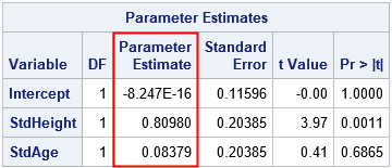
The parameter estimates for the standardized data are equal to the STB estimates for the original data. Furthermore, the t values and p-values for the slope parameters are equivalent because these statistics are scale- and translation-invariant. Notice, however, that scale-dependent statistics such as standard errors and covariance of the betas will not be the same for the two analyses.
Linear transformations of random variables
Mathematically, you can use a algebra to understand how linear transformations affect the relationship between two linearly dependent random variables. Suppose X is a random variable and Y = b0 + b1*X for some constants b0 and b1. What happens to this linear relationship if you apply linear transformations to X and Y?
Define new variables
U = (Y - cY) / sY and
V = (X - cX) / sX. If you solve for X and Y and plug the expressions into the equation for the linear relationship, you find that the new random variables are related by
U = (b0 + b1*cX - cY) / sY + b1*(sX/sY)*V.
If you define B0 = (b0 + b1*cX - cY) / sY
and B1 = b1*(sX/sY), then U = B0 + B1*V, which shows that the transformed variables (U and V) are linearly related.
The physical significance of this result is that linear relationships persist no matter what units you choose to measure the variables. For example, if X is measured in inches and Y is measured in pounds, then the quantities remain linearly related if you measure X in centimeters and measure Y in "kilograms from 20 kg."
The effect of standardizing variables on regression estimates
The analysis in the previous section holds for any linear transformation of linearly related random variables. But suppose, in addition, that
- U and V are standardized versions of Y and X, respectively. That is, cY and cX are the sample means and sY and sX are the sample standard deviations.
- The parameters b0 and b1 are the regression estimates for a simple linear regression model.
For simple linear regression, the intercept estimate is b0 = cY - b1*cY, which implies that B0 = 0. Furthermore, the coefficient B1 = b1*(sX/sY) is the original parameter estimate "divided by the ratio of the sample standard deviation of the dependent variable to the sample standard deviation of the regressor," just as the PROC REG documentation states and just as we saw in the PROC REG output in the previous section. Thus the STB option on the MODEL statement does not need to standardize any data! It produces the standardized estimates by setting the intercept term to 0 and dividing the parameter estimates by the ratio of standard deviations, as noted in the documentation. (A similar proof handles multiple explanatory variables.)
Interpretation of the regression coefficients
For the original (unstandardized) data, the intercept estimate predicts the value of the response when the explanatory variables are all zero. The regression coefficients predict the change in the response for one unit change in an explanatory variable while holding the other variables at a constant value. ("Holding at a constant value" is sometimes called "controlling for the other variables in the model.") The "change in response" depends on the units for the data, such as kilograms per centimeter.
The standardized coefficients predict the number of standard deviations that the response will change for one STANDARD DEVIATION of change in an explanatory variable. The "change in response" is a unitless quantity. The fact that the standardized intercept is 0 indicates that the predicted value of the (centered) response is 0 when the model is evaluated at the mean values of the explanatory variables.
In summary, standardized coefficients are the parameter estimates that you would obtain if you standardize the response and explanatory variables by centering and scaling the data. A standardized parameter estimate predicts the change in the response variable (in standard deviations) for one standard deviation of change in the explanatory variable (while controlling for the other variables).

21 Comments
Hi Rick,
Thanks for another great blog post. I have a couple of questions:
1. The SAS documentation states that the STB for class variables is dependent on the coding of the classification variable - meaning that the STB estimate can easily be manipulated simply by coding the class variable differently. Is there any way to overcome this inconsistency?
2. In proc phreg the STB option is not available. However, since SAS 9.4M4, proc phreg allows for compuation of the ROC for time event outcomes, e.g. Harrel's C-index for all-cause mortality at 10-years. As I understand the problem of censoring is overcome by inverse probability censoring weights, which means that all individuals are assigned a yes/no to the outcome variable. Thus, it should be possible to extend the STB option to proc phreg?
Thanks again
1. I wouldn't say they are "easily manipulated." Yes, using CLASS variables requires making a choice of parameterization, which determines the dummy variables (columns) in a design matrix. So each choice results in a different set of standardized variables and coefficients. Just be sure to specify the parameterization when you report the coefficients, just as you must do with the raw (unstandardized) values.
2. I don't know. You can ask SAS Technical Support or a discussion forum like Stack Overflow.
Thanks for this clear demonstration and explanation. Could parts of it go in the documentation?
Great post! How would you interpret standardized coefficient estimates for interaction terms. For example, Y is regressed on X1, X2, and X1*X2.
Interpretation of interaction effects is always a challenge. If you know how to do it for the original variables, the basic idea is the same except now the variables are measured from a different baseline and in different units.
I would like to see some full examples using standardized vars to construct polynomial models with complete instructions, with examples on how to transform the parameters back. The examples you give sound right, but there are too many ways to interpret this to trust applying it. For that reason, it would help me to see an example of data that is transformed, regressed, and transformed back along with transformed parameter estimates. Thanks.
If it helps, I have written two examples that demonstrate how to change from one basis to another:
Regression coefficients in different bases
Regression coefficients for orthogonal polynomials
If those articles are not sufficient, then you might want to post this question (with additional details) to a forum such as CrossValidated.
Thanks for this explanation in the post. Could these stb and select options also be used in the phreg statement? Thank you.
The STB option is not supported by PROC PHREG. The ODS SELECT statement is a global statement so you can use it with all SAS procedures.
Great post! How would you obtain confidence intervals for the standardized estimates or stb option in proc reg?
The easiest way is to add the CLB option to the second PROC REG step, the one that uses the standardized data.
Rick,
I am enjoying your posts for years, thank you for many practical hints.
My question: p
In logistic regression we analyze sometimes required to derive standardized estimator. Jon Arni Steingrimssona, Daniel F. Hanleyb, Michael Rosenblum in "Improving precision by adjusting for prognostic baseline variables in randomized trials with binary outcomes, without regression model assumptions" (2017) recommend a specific algorithm for a standardized estimator (page 20). Does SAS stat package have the capability to derive these, are there any ready to use macros or options?
I don't see a page 20, but perhaps you are talking about Appendix A, which starts after page 19. I am not aware of any existing SAS code, but it would not be hard to implement it yourself. It looks like the computation scores the model on two disjoint data sets, computes the average predicted probabilities and forms the difference.
Hi Rick, Thanks for this great blog post. I am running a logistic regression and will be presenting the standardized coefficients as part of my results.
Can you tell me if the interpretation of standardized coefficients is the same for logistic regression as it is for linear regression? Your blog post has an example of linear regression, and states this: "The standardized coefficients predict the number of standard deviations that the response will change for one STANDARD DEVIATION of change in an explanatory variable. The "change in response" is a unitless quantity. The fact that the standardized intercept is 0 indicates that the predicted value of the (centered) response is 0 when the model is evaluated at the mean values of the explanatory variables."
Can I use the same interpretation for logistic regression? Thanks very much.
You cannot use the same interpretation because the predicted response is a probability, which is bounded on [0,1]. I think the interpretation is:
the number of standard deviations that the LOG ODDS of the response will change for one standard deviation of change in an explanatory variable.
Agree, probably not too difficult, point is, the algorithm in section 2 is expected to be very frequently used maybe SAS should consider adding this utility? (or at least this could be a great The Do Loop next topic?)
SAS does offer the macro afterall: https://support.sas.com/kb/63/038.html
It would be nice to see a post on the STDCOEF option in PROC GLIMMIX
I have the same question. I would expect that the STB option from Proc Reg should be equivalent to the STDCOEF option in GLIMMIX (for dist=normal, link=identity), but I get different results. Perhaps I'm misunderstanding what STDCOEF yields.
See the formula for the NOCENTER option in PROC GLIMMIX. It shows how GLIMMIX standardizes the columns of the design matrix. Therefore, the following are equivalent:
1. For the raw data, use the STDCOEF option on the MODEL statement.
2. Standardize the data by using (x-mean(x))/sqrt(CSS). Estimate the fixed effects without using the STDCOEF option.
Pingback: Standardized regression coefficients in PROC GLIMMIX - The DO Loop