SAS enables you to evaluate a regression model at any location within the range of the data. However, sometimes you might be interested in how the predicted response is increasing or decreasing at specified locations. You can use finite differences to compute the slope (first derivative) of a regression model. This numerical approximation technique is most useful for nonparametric regression models that cannot be simply written in terms of an analytical formula.
A nonparametric model of drug absorption
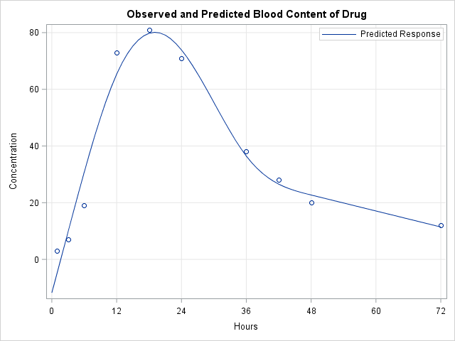
The following data are the hypothetical concentrations of a drug in a patient's bloodstream at times (measured in hours) during a 72-hour period after the drug is administered. For a real drug, a pharmacokinetic researcher might construct a parametric model and fit the model by using PROC NLMIXED. The following example uses the EFFECT statement to fit a regression model that uses cubic splines. Other nonparametric models in SAS include loess curves, generalized additive models, adaptive regression, and thin-plate splines.
data Drug; input Time Concentration @@; datalines; 1 3 3 7 6 19 12 73 18 81 24 71 36 38 42 28 48 20 72 12 ; proc glmselect data=Drug; effect spl = spline(Time/ naturalcubic basis=tpf(noint) knotmethod=percentiles(5)); model Concentration = spl / selection=none; /* fit model by using spline effects */ store out=SplineModel; /* store model for future scoring */ quit; |
Because the data are not evenly distributed in time, a graph of the spline fit evaluated at the data points does not adequately show the response curve. Notice that the call to PROC GLMSELECT used a STORE statement to store the model to an item store. You can use PROC PLM to score the model on a uniform grid of values to visualize the regression model:
/* use uniform grid to visualize curve */ data ScoreData; do Time = 0 to 72; output; end; run; /* score the model on the uniform grid */ proc plm restore=SplineModel noprint; score data=ScoreData out=ScoreResults; run; /* merge fitted curve with original data and plot the fitted curve */ data All; set Drug ScoreResults; run; title "Observed and Predicted Blood Content of Drug"; proc sgplot data=All noautolegend; scatter x=Time y=Concentration; series x=Time y=Predicted / name="fit" legendlabel="Predicted Response"; keylegend "fit" / position=NE location=inside opaque; xaxis grid values=(0 to 72 by 12) label="Hours"; yaxis grid; run; |
Finite difference approximations for derivatives of nonparametric models
A researcher might be interested in knowing the slope of the regression curve at certain time points. The slope indicates the rate of change of the response variable (the blood-level concentration). Because nonparametric regression curves do not have explicit formulas, you cannot use calculus to compute a derivative. However, you can use finite difference formulas to compute a numerical derivative at any point.
There are several finite difference formulas for the first derivative. The forward and backward formulas are less accurate than the central difference formula. Let h be a small value. Then the approximate derivative of a function f at a point t is given by
f′(t) ≈ [ f(t + h) – f(t – h) ] / 2h
/* compute derivatives at specified points */ data ScoreData; h = 0.5e-5; do t = 6 to 48 by 6; /* siz-hour intervals */ Time = t - h; output; Time = t + h; output; end; keep t Time h; run; /* score the model at each time point */ proc plm restore=SplineModel noprint; score data=ScoreData out=ScoreOut; /* Predicted column contains f(x+h) and f(x-h) */ run; /* compute first derivative by using central difference formula */ data Deriv; set ScoreOut; Slope = dif(Predicted) / (2*h); /* [f(x+h) - f(x-h)] / 2h */ Time = t; /* estimate slope at this time */ if mod(_N_,2)=0; /* process observations in pairs; keep even obs */ drop h t; run; proc print data=Deriv; run; |
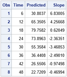
The output shows that after six hours the drug is entering the bloodstream at 6.8 units per hour. By 18 hours, the rate of absorption has slowed to 0.6 units per hour. After 24 hours, the rate of absorption is negative, which means that the blood-level concentration is decreasing. At approximately 30 hours, the drug is leaving the bloodstream at the rate of -3.5 units per hour.
This technique generalizes to other nonparametric models. If you can score the model, you can use the central difference formula to approximate the first derivative in the interior of the data range.
For more about numerical derivatives, including a finite-difference approximation of the second derivative, see Warren Kuhfeld's article on derivatives for penalized B-splines. Warren's article is focused on how to obtain the predicted values that are generated by the built-in regression models in PROC SGPLOT (LOESS and PBSPLINE), but it contains derivative formulas that apply to any regression curve.

7 Comments
Rick,
/* process observations in pairs; drop even obs */
Should be
/* process observations in pairs; keep even obs */
?
Yes, thanks. I have updated that comment.
Thank you for sharing the post, Rick.
When creating the 'ScoreData', my multivariable model contains categorical and continuous predictors. For each predictor, how do I determine which values to input? In your above example for instance, if the predictors sex (binary) and birth weight (continuous) were in your model, what values would be specified after the datastep: do Time = 0 to 72;
Thank you for your help!
You are asking about how to slice the regression surface when there are multiple explanatory variables. For your example, if MIN is the minimum weight and MAX is the maximum weight, you can visualize the model by creating the following scoring values:
Thank you very much for your time and sharing these additional details, Rick, I really appreciate it! I reviewed your article on how to slice the regression surface - I think this may be more advanced than what I am trying to visualize. I am hoping to visualize my multivariable regression model, with the inclusion of splines for my primary exposure of interest. To achieve this, would it be appropriate for me to create scoring values for each of my model covariates as you show above, and then plot the fitted curve using proc plm and sgplot?
Sure, you can do that. Also, some SAS procedures can create a fitplot automatically if you use the PLOTS= option on the PROC statement. See
"How to create a sliced fit plot in SAS."
Thank you, Rick, you have been very helpful!!
All the best,
Adele