When you fit nonlinear fixed-effect or mixed models, it is difficult to guess the model parameters that fit the data. Yet, most nonlinear regression procedures (such as PROC NLIN and PROC NLMIXED in SAS) require that you provide a good guess! If your guess is not good, the fitting algorithm, which is often a nonlinear optimization algorithm, might not converge. This seems to be a Catch-22 paradox: You can't estimate the parameters until you fit the model, but you can't fit the model until you provide an initial guess!
Fortunately, SAS provides a way to circumvent this paradox: you can specify multiple initial parameter values for the nonlinear regression models in PROC NLIN and PROC NLMIXED. The procedure will evaluate the model on a grid that results from all combinations of the specified values and initialize the optimization by using the value in the grid that provides the best fit. This article shows how to specify a grid of initial values for a nonlinear regression model.
An example that specifies a grid of initial values
The following data and model is from the documentation of the NLMIXED procedure. The data describe the number of failures and operating hours for 10 pumps. The pumps are divided into two groups: those that are operated continuously (group=1) and those operated intermittently (group=2). The number of failures is modeled by a Poisson distribution whose parameter (lambda) is fit by a linear regression with separate slopes and intercepts for each group. The example in the documentation specifies a single initial value (0 or 1) for each of the five parameters. In contrast, the following call to PROC NLMIXED specifies multiple initial values for each parameter:
data pump; input y t group;q pump = _n_; logtstd = log(t) - 2.4564900; datalines; 5 94.320 1 1 15.720 2 5 62.880 1 14 125.760 1 3 5.240 2 19 31.440 1 1 1.048 2 1 1.048 2 4 2.096 2 22 10.480 2 ; proc nlmixed data=pump; parms logsig 0 1 /* multiple initial guesses for each parameter */ beta1 -1 to 1 by 0.5 beta2 -1 to 1 by 0.5 alpha1 1 5 10 alpha2 1 5; /* use BEST=10 option to see top 10 choices */ if (group = 1) then eta = alpha1 + beta1*logtstd + e; else eta = alpha2 + beta2*logtstd + e; lambda = exp(eta); model y ~ poisson(lambda); random e ~ normal(0,exp(2*logsig)) subject=pump; run; |
On the PARMS statement, several guesses are provided for each parameter. Two or three guesses are listed for the logsig, alpha1, and alpha2 parameters. An arithmetic sequence of values is provided for the beta1 and beta2 parameters. The syntax for an arithmetic sequence is start TO stop BY increment, although you can omit the BY clause if the increment is 1. In this example, the arithmetic sequence is equivalent to the list -1, -0.5, 0, 0.5, 1.
The procedure will form the Cartesian product of the guesses for each parameter. Thus the previous syntax specifies a uniform grid of points in parameter space that contains 2 x 5 x 5 x 3 x 2 = 300 initial guesses. As this example indicates, the grid size grows geometrically with the number of values for each parameter. Therefore, resist the urge to use a fine grid for each parameter. That will result in many unnecessary evaluations of the log-likelihood function.
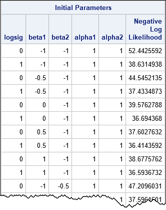
The following table shows a few of the 300 initial parameter values, along with the negative log-likelihood function evaluated at each set of parameters. From among the 300 initial guesses, the procedure will find the combination that results in the smallest value of the negative log-likelihood function and use that value to initialize the optimization algorithm.
If you want to visualize the range of values for the log-likelihood function, you can graph the negative log-likelihood versus the row number. In the following graph, a star indicates the parameter value in the grid that has the smallest value of the negative log-likelihood. I used the IMAGEMAP option on the ODS GRAPHICS statement to turn on tool tips for the graph, so that the parameter values for each point appears when you hover the mouse pointer over the point.
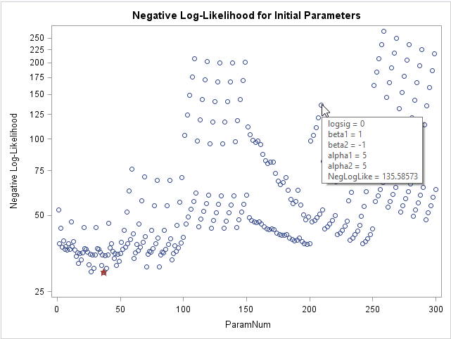
The graph shows that about 10 parameter values have roughly equivalent log-likelihood values. If you want to see those values in a table, you can add the BEST=10 option on the PARMS statement. In this example, there is little reason to choose the smallest parameter value over some of the other values that have a similar log-likelihood.
Create a file for the initial parameters
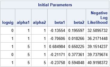
The ability to specify lists and arithmetic sequences is powerful, but sometimes you might want to use parameter values from a previous experiment or study or from a simplified model for the data. Alternatively, you might want to generate initial parameter values randomly from a distribution such as the uniform, normal, or exponential distributions. The PARMS statement in PROC NLMIXED supports a DATA= option that enables you to specify a data set for which each row is a set of parameter values. (In PROC NLIN and other SAS procedures, use the PDATA= option.) For example, the following DATA step specifies two or three values for the logsig, alpha1, and alpha2 parameters. It specifies random values in the interval (-1, 1) for the beta1 and beta2 parameters. The ParamData data set has 12 rows. The NLMIXED procedure evaluates the model on these 12 guesses, prints the top 5, and then uses the best value to initialize the optimization algorithm:
data ParamData; call streaminit(54321); do logsig = 0, 1; do alpha1 = 1, 5, 10; do alpha2 = 1, 5; beta1 = -1 + 2*rand("uniform"); /* beta1 ~ U(-1, 1) */ beta2 = -1 + 2*rand("uniform"); /* beta2 ~ U(-1, 1) */ output; end; end; end; run; proc nlmixed data=pump; parms / DATA=ParamData BEST=5; /* read guesses for parameters from data set */ if (group = 1) then eta = alpha1 + beta1*logtstd + e; else eta = alpha2 + beta2*logtstd + e; lambda = exp(eta); model y ~ poisson(lambda); random e ~ normal(0,exp(2*logsig)) subject=pump; run; |
As mentioned, the values for the parameters can come from anywhere. Sometimes random values are more effective than values on a regular grid. If you use a BOUNDS statement to specify valid values for the parameters, any infeasible parameters are discarded and only feasible parameter values are used.
Summary
In summary, this article provides an example of a syntax to specify a grid of initial parameters. SAS procedures that support a grid search include NLIN, NLMIXED, MIXED and GLIMMIX (for covariance parameters), SPP, and MODEL. You can also put multiple guesses into a "wide form" data set: the names of the parameters are the columns and each row contains a different combination of the parameters.
It is worth emphasizing that if your model does not converge, it might not be the parameter search that is at fault. It is more likely that the model does not fit your data. Although the technique in this article is useful for finding parameters so that the optimization algorithm converges, no technique cannot compensate for an incorrect model.

3 Comments
Great post Rick!
I'm trying to do a simple profile marginal likelihood, for the parameters of the covariance with nlmixed.
It's very easy to get the output in glimmix and mixed with COVTEST (to obtain statistical inferences for the covariance parameters).
Specifically, I'm trying to get the loglikelihood to be able to plot the marginal profile likelihood of the covariance parameter elements.
It seems in the manual of NLMIXED that CovMatParmEst, is the way to go, but I cannot get an evaluation of the probability of each parameter value in the grid.
Using your example :
ods output ParameterEstimates=pe
ConvergenceStatus=p2
CovMatAddEstCorrMatAddEst=p3
CorrMatParmEst=p4
CovMatAddEst=p5
CovMatParmEst=p6;
proc nlmixed data=pump ECORR CORR ECOV COV EDER;
parms logsig=0 to 1 by .1; /* read guesses for parameters from data set */
if (group = 1) then
eta = alpha1 + beta1*logtstd + e;
else eta = alpha2 + beta2*logtstd + e;
lambda = exp(eta);
model y ~ poisson(lambda);
random e ~ normal(0,exp(2*logsig)) subject=pump;
run;
I'm able to get pe, p2, p4, p6. But not p3 or p5.
Am I pointing in the right direction?
You can ask SAS programming questions at the SAS Support Communities.
Pingback: The DOLIST syntax: Specify a list of numerical values in SAS - The DO Loop