Data analysts often fit a probability distribution to data. When you have access to the data, a common technique is to use maximum likelihood estimation (MLE) to compute the parameters of a distribution that are "most likely" to have produced the observed data. However, how can you fit a distribution if you do not have access to the data?
This question was asked by a SAS programmer who wanted to fit a gamma distribution by using sample quantiles of the data. In particular, the programmer said, "we have the 50th and 90th percentile" of the data and "want to find the parameters for the gamma distribution [that fit] our data."
This is an interesting question. Recall that the method of moments uses sample moments (mean, variance, skewness,...) to estimate parameters in a distribution. When you use the method of moments, you express the moments of the distribution in terms of the parameters, set the distribution's moments equal to the sample moments, and solve for the parameter values for which the equation is true.
In a similar way, you can fit a distribution matching quantiles: Equate the sample and distributional quantiles and solve for the parameters of the distribution. This is sometimes called quantile-matching estimation (QME). Because the quantiles involve the cumulative distribution function (CDF), the equation does not usually have a closed-form solution and must be solved numerically.
Fit a two-parameter distribution from two quantiles
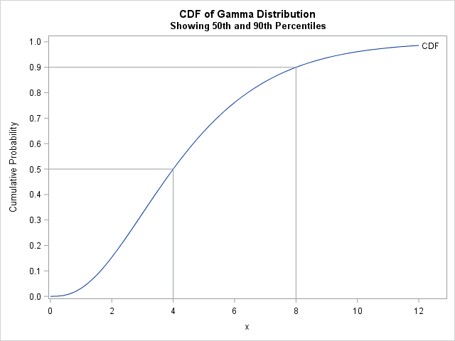
To answer the programmer's question, suppose you do not have the original data, but you are told that the 50th percentile (median) of the data is x = 4 and the 90th percentile is x = 8. You suspect that the data are distributed according to a gamma distribution, which has a shape parameter (α) and a scale parameter (β). To use quantile-matching estimation, set F(4; α, β) = 0.5 and F(8; α, β) = 0.9, where F is the cumulative distribution of the Gamma(α, β) distribution. You can then solve for the values of (α, β) that satisfy the equations. You will get a CDF that matches the quantiles of the data, as shown to the right.
I have previously written about four ways to solve nonlinear equations in SAS. One way is to use PROC MODEL, as shown below:
data initial; alpha=1; beta=1; /* initial guess for finding root */ p1=0.5; X1 = 4; /* eqn for 1st quantile: F(X1; alpha, beta) = p1 */ p2=0.9; X2 = 8; /* eqn for 2nd quantile: F(X2; alpha, beta) = p2 */ run; proc model data=initial; eq.one = cdf("Gamma", X1, alpha, beta) - p1; /* find root of eq1 */ eq.two = cdf("Gamma", X2, alpha, beta) - p2; /* and eq2 */ solve alpha beta / solveprint out=solved outpredict; run;quit; proc print data=solved noobs; var alpha beta; run; |
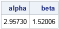
The output indicates that the parameters (α, β) = (2.96, 1.52) are the values for which the Gamma(α, β) quantiles match the sample quantiles. You can see this by graphing the CDF function and adding reference lines at the 50th and 90th percentiles, as shown at the beginning of this section. The following SAS code creates the graph:
/* Graph the CDF function to verify that the solution makes sense */ data Check; set solved; /* estimates of (alpha, beta) from solving eqns */ do x = 0 to 12 by 0.2; CDF = cdf("gamma", x, alpha, beta); output; end; run; title "CDF of Gamma Distribution"; title2 "Showing 50th and 90th Percentiles"; proc sgplot data=Check; series x=x y=CDF / curvelabel; dropline y=0.5 X=4 / dropto=both; /* first percentile */ dropline y=0.9 X=8 / dropto=both; /* second percentile */ yaxis values=(0 to 1 by 0.1) label="Cumulative Probability"; xaxis values=(0 to 12 by 2); run; |
Least squares estimates for matching quantiles
The previous section is relevant when you have as many sample quantiles as parameters. If you have more sample quantiles than parameters, then the system is overconstrained and you probably want to compute a least squares solution. If there are m sample quantiles, the least squares solution is the set of parameters that minimizes the sum of squares Σim (pi – F(xi; α, β))2.
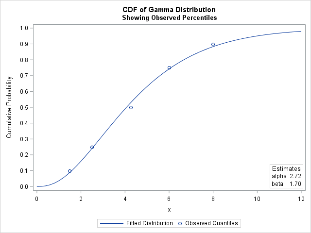
For example, the following DATA step contains five sample quantiles. The observation (p,q) = (0.1, 1.48) indicates that the 10th percentile is x=1.48. The second observation indicates that the 25th percentile is x=2.50. The last observation indicates that the 90th percentile is x=7.99. You can use PROC NLIN to find a least squares solution to the quantile-matching problem, as follows:
data SampleQntls; input p q; /* p is cumul probability; q is p_th sample quantile */ datalines; 0.1 1.48 0.25 2.50 0.5 4.25 0.75 6.00 0.9 7.99 ; /* least squares fit of parameters */ proc nlin data=SampleQntls /* sometimes the NOHALVE option is useful */ outest=PE(where=(_TYPE_="FINAL")); parms alpha 2 beta 2; bounds 0 < alpha beta; model p = cdf("Gamma", q, alpha, beta); run; proc print data=PE noobs; var alpha beta; run; |
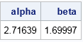
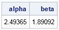
The solution indicates the parameter values (α, β) = (2.72, 1.70) minimize the sum of squares between the observed and theoretical quantiles. The following graph shows the observed quantiles overlaid on the CDF of the fitted Gamma(α, β) distribution. Alternatively, you can graph the quantile-quantile plot of the observed and fitted quantiles.
Weighted least squares estimates for matching quantiles
For small samples, quantiles in the tail of a distribution have a large standard error, which means that the observed quantile might not be close to the theoretical quantile. One way to handle that uncertainty is to compute a weighted regression analysis where each sample quantile is weighted by the inverse of its variance. According to Stuart and Ord (Kendall’s Advanced Theory of Statistics, 1994, section 10.10), the standard error of the p_th sample quantile in a sample of size n is σ2 = p(1-p) / (n f(ξp)2), where ξp is the p_th quantile of the distribution and f is the probability density function.
In PROC NLIN, you can perform weighted analysis by using the automatic variable _WEIGHT_. The following statements define the variance of the p_th sample quantile and define weights equal to the inverse variance. Notice the NOHALVE option, which can be useful for iteratively reweighted least squares problems. The option eliminates the requirement that the weighted sum of squares must decrease at every iteration.
/* weighted least squares fit where w[i] = 1/variance[i] */ proc nlin data=SampleQntls NOHALVE outest=WPE(where=(_TYPE_="FINAL")); parms alpha 2 beta 2; bounds 0 < alpha beta; N = 80; /* sample size */ xi = quantile("gamma", p, alpha, beta); /* quantile of distrib */ f = pdf("Gamma", xi, alpha, beta); /* density at quantile */ variance = p*(1-p) / (N * f**2); /* variance of sample quantiles */ _weight_ = 1 / variance; /* weight for each observation */ model p = cdf("Gamma", q, alpha, beta); run; |
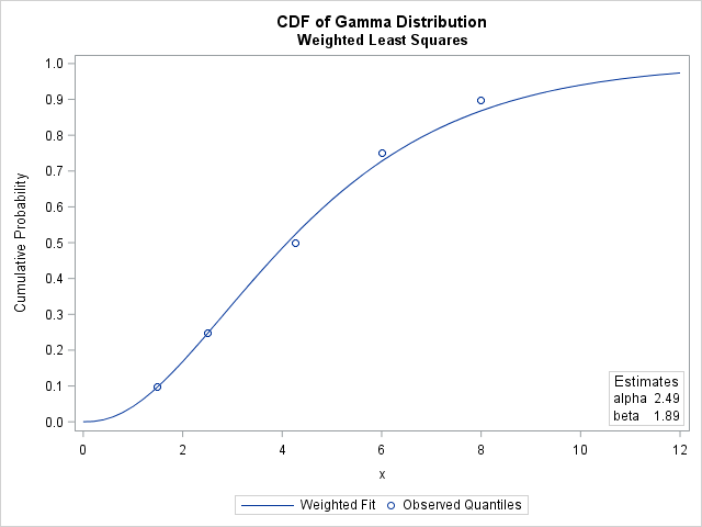
The parameter estimates for the weighted analysis are slightly different than for the unweighted analysis. The following graph shows the CDF for the weighted estimates, which does not pass as close to the 75th and 90th percentiles as does the CDF for the unweighted estimates. This is because the PDF of the gamma distribution is relatively small for those quantiles, which causes the regression to underweight those sample quantiles.
In summary, this article shows how to use SAS to fit distribution parameters to observed quantiles by using quantile-matching estimation (QME). If the number of quantiles is the same as the number of parameters, you can numerically solve for the parameters for which the quantiles of the distribution equal the sample quantiles. If you have more quantiles than parameters, you can compute a least squares estimate of the parameters. Because quantile estimates in the tail of a distribution have larger uncertainty, you might want to underweight those quantiles. One way to do that is to run a weighted least squares regression where the weights are inversely proportional to the variance of the sample quantiles.

11 Comments
IMHO the most obvious way to fit model parameters in presence of summaries of data (rather than actual data) is approximate Bayesian computation, e.g. https://arxiv.org/abs/1001.2058
Thanks for the comment. I passed it on to a colleague who knows about Bayesian analysis and he sent me the following comments and code regarding solving this problem with PROC MCMC in SAS:
Least square and MLE in normal likelihood are the same thing, so we can use a normal likelihood function, say, in NLMIXED:
which gives the same estimates as alpha and beta, 2.7164 and 1.700.
Now we can do the same thing in PROC MCMC, and use noninformative priors, flat on alpha and beta, Jeffreys’ on the variance. (Well, I don’t know if uniform on alpha and beta are noninformative in this case because they enter the model via the CDF function, but the Jeffreys’ prior on variance in a normal model is more of a safe bet).
This gives reasonable estimates to alpha and beta:
                                           Standard
     Parameter           N        Mean    Deviation      95% HPD Interval

     alpha           50000      2.7237       0.3567      1.9922      3.4810
     beta            50000      1.7331       0.2785      1.1881      2.2261
     s2              50000     0.00112      0.00203    0.000062     0.00360
If one is concerned with mixing due to the Jeffreys’ prior, we can use an inverse-gamma prior that mimics the Jeffreys’, with mean pushed very close to zero:
which effectively gave similar point estimates.
Standard Parameter N Mean Deviation 95% HPD Interval alpha 50000 2.7226 0.2028 2.3291 3.1454 beta 50000 1.7079 0.1393 1.4402 2.0068 s2 50000 0.000316 0.000247 0.000071 0.000737What is the easy way to fit newly developed distribution? SAS has not been friendly on this aspect. I am forced to go start learning R to do the computations necessary. For instance, Maximum product spacing and other estimation techniques are not captured in SAS. This is frustrating!
The easiest way if probably maximum likelihood estimation, which you can perform in SAS by using PROC NLMIXED or PROC IML.
Please Sir, can you give an example? I want to fit a newly developed compound distribution with SAS. An example using NLMIXED will be highly appreciated, thanks.
This article gives an example of fitting parameters from published quantiles. It sounds like you want to fit parameters from data.
You can do this by using the GENERAL loglikelihood of the distribution in PROC NLMIXED. If you have questions, post them to the SAS Support Communities.
Sir,
Will it be possible to fit quantile values for multivariate distribution as shown in the above code . I'm trying for 2 dimension dirichlet distribution but I guess in multivariate case problem of countours also comes in.
Does this really come up in practice? I've never seen a 2-D distribution described in terms of quantiles of the 2-D CDF.
I think that is a challenging problem. I suspect that it is theoretically possible, but I have never done it myself. The problem is that you need a way to specify the multivariate CDF, which does not have a closed-form solution for most multivariate distributions. For example, I do not know an equation for the 2-D Dirichlet CDF. You can, of course, integrate the PDF by using SAS/IML software. If the quantile is known at (x1,x2), then for each vector of shape parameters, you need to approximate the CDF at (x1,x2) by the double integral
CDF(x_1, x_2) = \int_0^{x_1} \int_0^{x_2} f(x_1, x_2; \alpha_0, \alpha_1, \alpha_2) dx_1 dx_2
where {\alpha_0, \alpha_1, \alpha_2} are the unknown parameter values that you want to solve for by some method, such as nonlinear least squares estimation.
I was wondering why maximum likelihood estimation is not mentioned much with regard to quantile matching estimation even though it's possible since you can estimate quantile sample variance using the formula given above p(1-p) / (n f(ξp)2) and figure it out from there assuming you also know the sample size. Then I did some testing and came to the conclusion that weighted least square is just as, if not more, good as maximum likelihood estimation in figuring out the true distribution parameter, perhaps due to some precision loss and numerical instability associated with this specific form of MLE (this was done using Python)
MLE is usually favored when you have a sample. MLE uses the probability density function to estimate the parameters of the distribution that is most likely to have given rise to the data. In contrast, this article assumes that the data are not available, but only summaries of the data. It shows how to fit the parameters of a model distribution to the summary statistics.
This is the MLE method I had in mind when I wrote my comment https://imgur.com/xU2K09h. It's a bit worse in terms of estimation accuracy compared to the weighted least squares solution for quantile matching estimation but I figured I should share because the more you know. Here's the link to the full code I wrote to estimate how well each method works https://github.com/cats256/assessment-statistics/blob/main/assessment-statistics/flask-server/log_likelihood.py