Your statistical software probably provides a function that computes quantiles of common probability distributions such as the normal, exponential, and beta distributions. Because there are infinitely many probability distributions, you might encounter a distribution for which a built-in quantile function is not implemented. No problem! This article shows how to numerically compute the quantiles of any continuous probability distribution from the definition of the cumulative distribution (CDF).

In SAS, the QUANTILE function computes the quantiles for about 25 distributions. This article shows how you can use numerical root-finding methods (and possibly numerical integration) in SAS/IML software to compute the quantile function for ANY continuous distribution. I have previously written about related topics and particular examples, such as the following:

• How to compute quantiles for the folded normal distribution
• How to compute quantiles for the contaminated normal distribution.
• How to compute quantiles for discrete probability distributions

The quantile is the root of an integral equation

Computing a quantile would make a good final exam question for an undergraduate class in numerical analysis. Although some distributions have an explicit CDF, many distributions are defined only by a probability density function (the PDF, f(x)) and numerical integration must be used to compute the cumulative distribution (the CDF, F(x)). A canonical example is the normal distribution. I've previously shown how to use numerical integration to compute a CDF from a PDF by using the definition F(x) = ∫ f(t) dt, where the lower limit of the integral is –∞ and the upper limit is x.

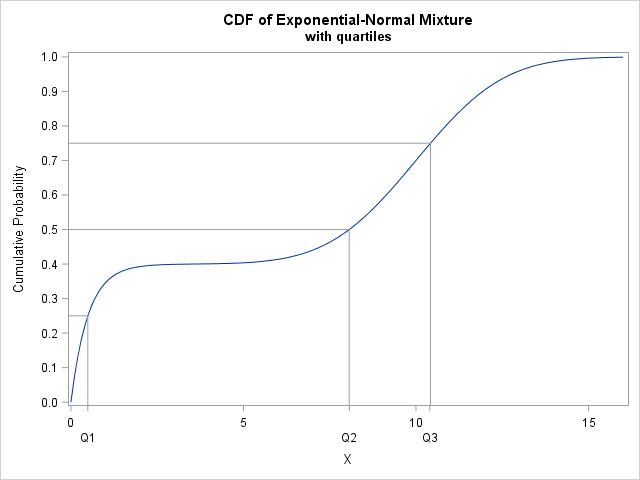
Whether the CDF is defined analytically or through numerical integration, the quantile for p is found implicitly as the solution to the equation F(x) = p, where p is a probability in the interval (0,1). This is illustrated by the graph at the right.

Equivalently, you can define G(x; p) = F(x) – p so that the quantile is the root of the equation G(x; p) = 0. For well-behaved densities that occur in practice, a numerical root is easily found because the CDF is monotonically increasing. (If you like pathological functions, see the Cantor staircase distribution.)

Example: Create a custom distribution

SAS/IML software provides the QUAD subroutine, which provides numerical integration, and the FROOT function, which solves for roots. Thus SAS/IML is an ideal computational environment for computing quantiles for custom continuous distributions.

As an example, consider a distribution that is a mixture of an exponential and a normal distribution:
F(x) = 0.4 F_exp(x; 0.5) + 0.6 Φ(x; 10, 2),
where F_exp(x; 0.5) is the exponential distribution with scale parameter 0.5 and Φ(x; 10, 2) is the normal CDF with mean 20 and standard deviation 2. In this case, you do not need to use numerical integration to compute the CDF. You can compute the CDF as a linear combination of the exponential and normal CDFs, as shown in the following SAS/IML function:

/* program to numerically find quantiles for a custom distribution */
proc iml;
/* Define the cumulative distribution function here. */
start CustomCDF(x); 
   F = 0.4*cdf("Exponential", x, 0.5) +
       0.6*cdf("Normal", x, 10, 2);
   return F;
finish;

The previous section shows the graph of the CDF on the interval [0, 16]. The vertical and horizontal lines correspond to the first, second and third quartiles of the distribution. The quartiles are close to the values Q1 ≈ 0.5, Q2 ≈ 8, and Q3 ≈ 10.5. The next section shows how to compute the quantiles.

Compute quantiles for an arbitrary continuous distribution

As long as you can define a function that evaluates the CDF, you can find quantiles. For unbounded distributions, it is usually helpful to plot the CDF so that you can visually estimate an interval that contains the quantile. (For bounded distributions, the support of the distribution contains all quantiles.) For the mixture distribution in the previous section, it is clear that the quantiles are in the interval [0, 16].

The following program finds arbitrary quantiles for whichever CDF is evaluated by the CustomCDF function. To find quantiles for a different function, you can modify the CustomCDF and change the interval on which to find the quantiles. You do not need to modify the RootFunc or CustomQuantile functions.

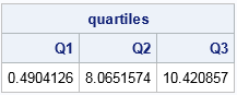
/* Express CDF(x)=p as the root for the function CDF(x)-p. */
start RootFunc(x) global(gProb);
   return CustomCDF(x) - gProb;  /* quantile for p is root of CDF(x)-p */
finish;
 
/* You need to provide an interval on which to search for the quantiles. */
start CustomQuantile(p, Interval) global(gProb);
   q = j(nrow(p), ncol(p), .);              /* allocate result matrix */
   do i = 1 to nrow(p)*ncol(p);             /* for each element of p... */
      gProb = p[i];                         /*    set global variable   */
      q[i] = froot("RootFunc", Interval);   /*    find root (quantile)  */ 
   end;
   return q;
finish;
 
/* Example: look for quartiles in interval [0, 16] */
probs = {0.25 0.5 0.75};         /* Q1, Q2, Q3 */
intvl = {0 16};                  /* interval on which to search for quantiles */
quartiles = CustomQuantile(probs, intvl);
print quartiles[colname={Q1 Q2 Q3}];

In summary, you can compute an arbitrary quantile of an arbitrary continuous distribution if you can (1) evaluate the CDF at any point and (2) numerically solve for the root of the equation CDF(x)-p for a probability value, p. Because the support of the distribution is arbitrary, the implementation requires that you provide an interval [a,b] that contains the quantile.

The computation should be robust and accurate for non-pathological distributions provided that the density is not tiny or zero at the value of the quantile. Although this example is illustrated in SAS, the same method will work in other software.