A statistical programmer read my article about the beta-binomial distribution and wanted to know how to compute the cumulative distribution (CDF) and the quantile function for this distribution. In general, if you know the PDF for a discrete distribution, you can also compute the CDF and quantile functions. This article shows how.
Continuous versus discrete distributions
Recall the four essential functions for any probability distribution: the probability density function (PDF), the cumulative distribution function (CDF), the quantile function, and the random-variate generator. SAS software provides the PDF, CDF, QUANTILE, and RAND function, which support for about 25 common families of distributions. However, there are infinitely many probability distributions. What can you do if you need a distribution that is not natively supported in SAS? The answer is that you can use tools in SAS (especially in SAS/IML software) to implement these functions yourself.
I have previously shown how to use numerical integration and root-finding algorithms to compute the CDF and quantile function for continuous distributions such as the folded normal distribution and the generalized Gaussian distribution. For discrete distributions, you can use a summation to obtain the CDF from the PDF. The CDF at X=x is the sum of the PDF values for all values of X that are less than or equal to x. The discrete CDF is a step function, so it does not have an inverse function. Given a probability, p, the quantile for p is defined as the smallest value of x for which CDF(x) ≥ p.
To simplify the discussion, assume that the random variable X takes values on the integers 0, 1, 2, .... Many discrete probability distributions in statistics satisfy this condition, including the binomial, Poisson, geometric, beta-binomial, and more.
Compute a CDF from a PDF
I will use SAS/IML software to implement the CDF and quantile functions. The following SAS/IML modules define the PDF function and the CDF function. If you pass in a scalar value for x, the CDF function computes the PDF from X=0 to X=x and sums up the individual probabilities. When x is a vector, the implementation is slightly more complicated, but the idea is the same.
proc iml; /* PMF function for the beta-binomial distribution. See https://blogs.sas.com/content/iml/2017/11/20/simulate-beta-binomial-sas.html */ start PDFBetaBinom(x, nTrials, a, b); logPMF = lcomb(nTrials, x) + logbeta(x + a, nTrials - x + b) - logbeta(a, b); return ( exp(logPMF) ); finish; /* CDF function for the beta-binomial distribution */ start CDFBetaBinom(x, nTrials, a, b); y = 0:max(x); /* all values of X less than max(x) */ PMF = PDFBetaBinom(y, NTrials, a, b); /* compute PMF(t) for t=0..max(x) */ cumPDF = cusum(PMF); /* cdf(T) = sum( PMF(t), t=0..T ) */ /* The input x can be a vector of values in any order. Use the LOC function to assign CDF(x) for each value of x */ CDF = j(nrow(x), ncol(x), .); /* allocate result (same size as x) */ u = unique(x); do i = 1 to ncol(u); /* for each unique value of x... */ idx = loc(x=u[i]); /* find the indices */ CDF[idx] = cumPDF[1+u[i]]; /* assign the CDF */ end; return CDF; finish; /* test the CDF function */ a = 6; b = 4; nTrials = 10; c = CDFBetaBinom(t, nTrials, a, b); |
Notice the computational trick that is used to compute the CDF for a vector of values. If you want to compute the CDF at two or more values (say X=5 and X=7), you can compute the PDF for X=0, 1, ... M where M is the maximum value that you need (such as 7). Along the way, you end up computing the CDF for all smaller values.
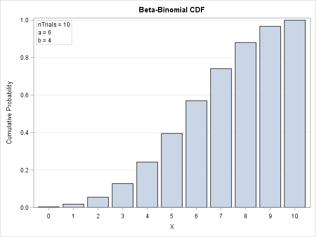
You can write the CDF values to a SAS data set and graph them to visualize the CDF of the beta-binomial distribution, as shown below:
Compute quantiles from the CDF
Given a probability value p, the quantile for p is smallest value of x for which CDF(x) ≥ p. Sometimes you can find a formula that enables you to find the quantile directly, but, in general, the definition of a quantile requires that you compute the CDF for X=0, 1, 2,... and so forth until the CDF equals or exceeds p.
The support of the beta-binomial distribution is the set {0, 1, ..., nTrials}. The following function first computes the CDF function for all values. It then looks at each value of p and returns the corresponding value of X that satisfies the quantile definition.
start QuantileBetaBinom(_p, nTrials, a, b); p = colvec(_p); /* ensure input is column vector */ y = 0:nTrials; /* all possible values of X */ CDF = CDFBetaBinom(y, NTrials, a, b); /* all possible values of CDF */ q = j(nrow(p), 1, .); /* allocate result vector */ do i = 1 to nrow(p); idx = loc( p[i] <= CDF ); /* find all x such that p <= CDF(x) */ q[i] = idx[1] - 1; /* smallest index. Subtract 1 from index to get x */ end; return ( q ); finish; p = {0.2, 0.5, 0.8}; q = QuantileBetaBinom(p, nTrials, a, b); print p q; |
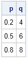
The output shows the quantile values for p = {0.2, 0.5, 0.8}. You can find the quantiles visually by using the graph of the CDF function, shown in the previous section. For each value of p on the vertical axis, draw a horizontal line until the line hits a bar. The x value of the bar is the quantile for p.
Notice that the QuantileBetaBinom function uses the fact that the beta-binomial function has finite support. The function computes the CDF at the values 0, 1, ..., nTrials. From those values you can "look up" the quantile for any p. If you have distribution with infinite support (such as the geometric distribution) or very large finite support (such as nTrials=1E9), it is more efficient to apply an iterative process such as bisection to find the quantiles.
Summary
In summary, you can compute the CDF and quantile functions for a discrete distribution directly from the PDF. The process was illustrated by using the beta-binomial distribution. The CDF at X=x is the sum of the PDF evaluated for all values less than x. The quantile for p is the smallest value of x for which CDF(x) ≥ p.

2 Comments
Hi Rick,
We do not have Proc IML, how hard is it to code the same process in Base SAS?
thanks
It should be straightforward (but less efficient) to use PROC FCMP to define the functions. Each call to the CDF will have to recompute the cumulative PDF from 0 to x. For the quantile, you can just accumulate the PDF until the cumulative sum exceeds p.