This article shows how to simulate beta-binomial data in SAS and how to compute the density function (PDF). The beta-binomial distribution is a discrete compound distribution. The "binomial" part of the name means that the discrete random variable X follows a binomial distribution with parameters N (number of trials) and p, but there is a twist: The parameter p is not a constant value but is a random variable that follows the Beta(a, b) distribution.
The beta-binomial distribution is used to model count data where the counts are "almost binomial" but have more variance than can be explained by a binomial model. Therefore this article also compares the binomial and beta-binomial distributions.
Simulate data from the beta-binomial distribution
To generate a random value from the beta-binomial distribution, use a two-step process. The first step is to draw p randomly from the Beta(a, b) distribution. Then you draw x from the binomial distribution Bin(p, N). The beta-binomial distribution is not natively supported by the RAND function SAS, but you can call the RAND function twice to simulate beta-binomial data, as follows:
/* simulate a random sample from the beta-binomial distribution */ %let SampleSize = 1000; data BetaBin; a = 6; b = 4; nTrials = 10; /* parameters */ call streaminit(4321); do i = 1 to &SampleSize; p = rand("Beta", a, b); /* p[i] ~ Beta(a,b) */ x = rand("Binomial", p, nTrials); /* x[i] ~ Bin(p[i], nTrials) */ output; end; keep x; run; |
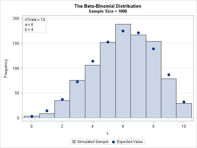
The result of the simulation is shown in the following bar chart. The expected values are overlaid. The next section shows how to compute the expected values.
The PDF of the beta-binomial distribution
The Wikipedia article about the beta-binomial distribution contains a formula for the PDF of the distribution. Since the distribution is discrete, some references prefer to use "PMF" (probability mass function) instead of PDF. Regardless, if X is a random variable that follows the beta-binomial distribution then the probability that X=x is given by
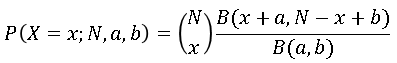
where B is the complete beta function.
The binomial coefficients ("N choose x") and the beta function are defined in terms of factorials and gamma functions, which get big fast. For numerical computations, it is usually more stable to compute the log-transform of the quantities and then exponentiate the result. The following DATA step computes the PDF of the beta-binomial distribution. For easy comparison with the distribution of the simulated data, the DATA step also computes the expected count for each value in a random sample of size N. The PDF and the simulated data are merged and plotted on the same graph by using the VBARBASIC statement in SAS 9.4M3. The graph was shown in the previous section.
data PDFBetaBinom; /* PMF function */ a = 6; b = 4; nTrials = 10; /* parameters */ do x = 0 to nTrials; logPMF = lcomb(nTrials, x) + logbeta(x + a, nTrials - x + b) - logbeta(a, b); PMF = exp(logPMF); /* probability that X=x */ EX = &SampleSize * PMF; /* expected value in random sample */ output; end; keep x PMF EX; run; /* Merge simulated data and PMF. Overlay PMF on data distribution. */ data All; merge BetaBin PDFBetaBinom(rename=(x=t)); run; title "The Beta-Binomial Distribution"; title2 "Sample Size = &SampleSize"; proc sgplot data=All; vbarbasic x / barwidth=1 legendlabel='Simulated Sample'; /* requires SAS 9.4M3 */ scatter x=t y=EX / legendlabel='Expected Value' markerattrs=GraphDataDefault(symbol=CIRCLEFILLED size=10); inset "nTrials = 10" "a = 6" "b = 4" / position=topleft border; yaxis grid; xaxis label="x" integer type=linear; /* force TYPE=LINEAR */ run; |
Compare the binomial and beta-binomial distributions
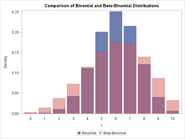
One application of the beta-binomial distribution is to model count data that are approximately binomial but have more variance ("thicker tails") than the binomial model predicts. The expected value of a Beta(a, b) distribution is a/(a + b), so let's compare the beta-binomial distribution to the binomial distribution with p = a/(a + b).
The following graph overlays the two PDFs for a = 6, b = 4, and nTrials = 10. The blue distribution is the binomial distribution with p = 6/(6 + 4) = 0.6. The pink distribution is the beta-binomial. You can see that the beta-binomial distribution has a shorter peak and thicker tails than the corresponding binomial distribution. The expected value for both distributions is 6, but the variance of the beta-binomial distribution is greater. Thus you can use the beta-binomial distribution as an alternative to the binomial distribution when the data exhibit greater variance than expected under the binomial model (a phenomenon known as overdispersion).
Summary
The beta-binomial distribution is an example of a compound distribution. You can simulate data from a compound distribution by randomly drawing the parameters from some distribution and then using those random parameters to draw the data. For the beta-binomial distribution, the probability parameter p is drawn from a beta distribution and then used to draw x from a binomial distribution where the probability of success is the value of p. You can use the beta-binomial distribution to model data that have greater variance than expected under the binomial model.
My next blog post shows how to compute the CDF and quantiles for the beta-binomial distribution.

9 Comments
For calculating the pmf for displaying expected frequencies in the histogram, you assume that the number of Bernoulli trials AND the parameters a and b are known quantities. Of course, when presented with data believed to come from a beta-binomial distribution, the parameters a and b will typically need to be estimated. Even though specified here as a parameter of the beta-binomial distribution, the number of Bernoulli trials will generally be known. When the number of trials are known, the parameters a and b can be estimated. The Wikipedia entry on the beta-binomial distribution mentions both moment estimators of a and b and also states that one can employ likelihood maximization to estimate the unknown parameters. Note that estimation through likelihood maximization allows the parameters themselves to depend on predictor variables . We do not have predictor variables in the example provided. But should predictor variables exist, the ability to allow the parameters to depend on covariates is beneficial.
Below, I present NLMIXED code that produces ML estimates of the parameters a and b. The NLMIXED procedure also computes the expected frequency under the beta-binomial distribution. There is no need for a data step to produce the expected frequencies. The parameter estimates are read in a data step and written to macro variables that are subsequently referenced as &a. and &b. in the SGPLOT procedure.
Note that the default NLMIXED likelihood maximization procedure (QUANEW) produced estimates of the parameters but did not produce standard errors for the parameter estimates. For these data, the DBLDOG maximization technique produced estimates with confidence intervals that contain the true parameters. Other data may require a different likelihood maximization technique.
Note, too, that the parameters a and b must be positive. Consequently, the NLMIXED procedure is parameterized in terms of log_a and log_b. Those parameters are exponentiated to produce a and b which are passed into the log-likelihood computation. Should a and b depend on covariates, the code expressed as "a = exp(log_a)" could be rewritten as "a = exp(b0_a + b1_a*X1 + b2_a*X2 ...;" with similar code for parameter b.
Thanks for writing and for including the code for the MLE estimates. I like the trick of using the parameters on the log scale. Readers who want to learn more about how to use PROC NLMIXED for MLE can refer to the article "Two ways to compute maximum likelihood estimates in SAS."
Since you mentioned regression, I will mention that PROC FMM can support beta-binomial regression. It uses a different parameterization and does not directly estimate a and b, but only the mean value a/(a+b), which is often the quantity of interest. It also requires that the data be in events/trials syntax. If you keep the nTrials variable in the simulated data, you can run the following:
Rick. I'm trying to find help, getting beta (PROC GLIMMIX Beta distribution) back on original scale
PROC glimMIX;
CLASS Phase TRT DAY ID;
MODEL DMIBWnew = TRT|phase /dist=beta DDFM=KR SOLUTION;
Random DAY/residual SUBJECT=ID;
LSmeans trt /DIFF ADJUST=SIMULATE (REPORT SEED=121211) cl adjdfe=row;
RUN; Quit;
I see that you have posted your question to the SAS Support Community. That's the correct place to ask questions like this.
The NLMIXED code can be rewritten to use a parameterization like that employed by FMM. See the code below. Of course, FMM would be the preferred procedure most of the time. But if one needed to introduce random effects due to data clustering, one could modify the NLMIXED code to accommodate that. Note that this parameterization appears more robust than the previous parameterization in that the default likelihood estimation technique (QUANEW) produced estimates with standard errors. (The DBLDOG technique also returns estimates with standard errors.)
Note that parameters a and b in this formulation of the likelihood match parameters from the previous formulation except at the 5th significant digit of b. Moreover, the estimate for eta matches the intercept estimate from FMM through the 4 significant digits reported by each procedure. The scale (overdispersion) parameter differs by a single digit at the 6th significant digit.
Again, since FMM can estimate this same beta-binomial model, the only reason to keep the NLMIXED code in one's hip pocket would be if there were yet another source of overdispersion attributable to random effects associated with clustered data collection.
Very nice summary. Thanks for taking the time to share this information.
Rick and Dale,
How could I apply this Beta-Binomial distribution into Logistic Regression ?
Hi Rick,
suppose Yt=f(Xt ,Zt) .Here only Yt is observable but Xt and Zt are not observable-however both are random variables for a given t( and hence{Xt} and {Zt} can be considered as two unobservable time series .)Therefore the problem is to disentangle the effect of Xt and Zt from Yt
like KALCVS or KALDFF any subroutine or proc like SSM forPARTICLE FILTERING?
Best,
Kaushik
You can ask questions like this on the SAS Support COmmunities. Since this is related to time series, I suggest you post to the Forecasting and Econometrics Community.