The article "Fisher's transformation of the correlation coefficient" featured a Monte Carlo simulation that generated sample correlations from bivariate normal data. The simulation used three steps:
- Simulate B samples of size N from a bivariate normal distribution with correlation ρ.
- Use PROC CORR to compute the sample correlation matrix for each of the B samples.
- Use the DATA step to extract the off-diagonal elements from the correlation matrices.
After the three steps, you obtain a distribution of B sample correlation coefficients that approximates the sampling distribution of the Pearson correlation coefficient for bivariate normal data.
There is a simpler way to simulate the correlation estimates: You can directly simulate from the Wishart distribution. Each draw from the Wishart distribution is a sample covariance matrix for a multivariate normal sample of size N. If you convert that covariance matrix to a correlation matrix, you can immediately extract the off-diagonal elements, as shown in the following SAS/IML statements:
%let rho = 0.8; /* correlation for bivariate normal distribution */ %let N = 20; /* sample size */ %let NumSamples = 2500; /* number of simulated samples */ /* generate sample correlation coefficients by using Wishart distribution */ proc iml; call randseed(12345); NumSamples = &NumSamples; DF = &N - 1; /* X ~ N obs from MVN(0, Sigma) */ Sigma = {1 &rho, /* covariance for MVN samples */ &rho 1 }; S = RandWishart(NumSamples, DF, Sigma); /* each row is 2x2 scatter matrix. Cov is 1/DF * S */ Corr = j(NumSamples, 1); /* allocate vector for correlation estimates */ do i = 1 to nrow(S); /* convert to correlation; extract off-diagonal */ Corr[i] = cov2corr( shape(S[i,], 2, 2) )[1,2]; end; |
You can create a comparative histogram of the sample correlation coefficients. In the following graph, the histogram at the top of the panel displays the distribution of the simulated correlation coefficients from the three-step method. The bottom histogram displays the distribution of correlations coefficients that are generated from the Wishart distribution.
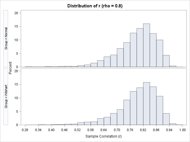
Visually, the histograms appear to be similar. You can use PROC NPAR1WAY to run various hypothesis tests that compare the distributions; all tests support the hypothesis that these two distributions are equivalent.
If you'd like to see the complete analysis, you can download the SAS program that runs both simulations and compares the resulting distributions.
Although the Wishart distribution is more efficient for this simulation, recall that the Wishart distribution assumes that the underlying data distribution is multivariate normal. In contrast, the three-step simulation is more general. It can be used to generate correlation coefficients for any data distribution. So although the three-step simulation is not necessary for multivariate normal data, it is still an important technique to store in your simulation toolbox.
