The singular value decomposition (SVD) could be called the "billion-dollar algorithm" since it provides the mathematical basis for many modern algorithms in data science, including text mining, recommender systems (think Netflix and Amazon), image processing, and classification problems. Although the SVD was mathematically discovered in the late 1800s, computers have made the SVD an indispensable tool in computational statistics and data science.
SVD: A fundamental theorem of linear algebra
Mathematically, the singular value decomposition is a fundamental theorem of linear algebra. )You could argue that it is THE fundamental theorem, but Gil Strang names a different result.) The singular value decomposition says that every n x p matrix can be written as the product of three matrices: A = U Σ VT where
- U is an orthogonal n x n matrix
- Σ is a diagonal n x p matrix. In practice, the diagonal elements are ordered so that Σii ≥ Σjj for all i < j.
- V is an orthogonal p x p matrix and VT represents a matrix transpose.
The SVD represents the essential geometry of a linear transformation. It tells us that every linear transformation is a composition of three fundamental actions. Reading the equation from right to left:
- The matrix V represents a rotation or reflection of vectors in the p-dimensional domain.
- The matrix Σ represents a linear dilation or contraction along each of the p coordinate directions. If n ≠ p, this step also canonically embeds (or projects) the p-dimensional domain into (or onto) the n-dimensional range.
- The matrix U represents a rotation or reflection of vectors in the n-dimensional range.
Thus the SVD specifies that every linear transformation is fundamentally a rotation or reflection, followed by a scaling, followed by another rotation or reflection. The Strang (1993) article about the fundamental theorem of linear algebra includes the following geometric interpretation of the singular value decomposition of a 2 x 2 matrix:
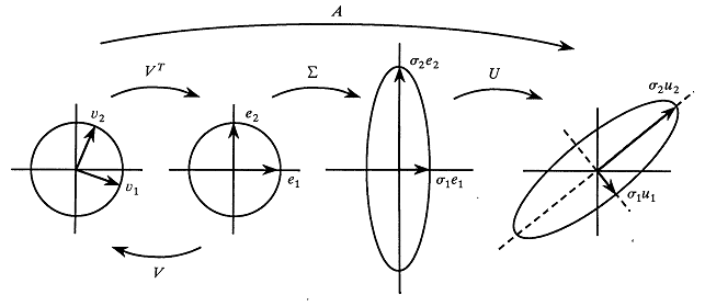
The diagram shows that the transformation induced by the matrix A (the long arrow across the top of the diagram) is equivalent to the composition of the three fundamental transformations, namely a rotation, a scaling, and another rotation.
SVD: The fundamental theorem of multivariate data analysis
Because of its usefulness, the singular value decomposition is a fundamental technique for multivariate data analysis. A common goal of multivariate data analysis is to reduce the dimension of the problem by choosing a small linear subspace that captures important properties of the data. The SVD is used in two important dimension-reducing operations:
- Low-rank approximations: Recall that the diagonal elements of the Σ matrix (called the singular values) in the SVD are computed in decreasing order. The SVD has a wonderful mathematical property: if you choose some integer k ≥ 1 and let D be the diagonal matrix formed by replacing all singular values after the k_th by 0, then then matrix U D VT is the best rank-k approximation to the original matrix A.
- Principal components analysis: The principal component analysis is usually presented in terms of eigenvectors of a correlation matrix, but you can show that the principal component analysis follows directly from the SVD. (In fact, you can derive the eigenvalue decomposition of a matrix, from the SVD.) The principal components of AT A are the columns of the V matrix; the scores are the columns of U. Dimension reduction is achieved by truncating the number of columns in U, which results in the best rank-k approximation of the data.
Compute the SVD in SAS
In SAS, you can use the SVD subroutine in SAS/IML software to compute the singular value decomposition of any matrix. To save memory, SAS/IML computes a "thin SVD" (or "economical SVD"), which means that the U matrix is an n x p matrix. This is usually what the data analyst wants, and it saves considerable memory in the usual case where the number of observations (n) is much larger than the number of variables (p). Technically speaking, the U for an "economical SVD" is suborthogonal: UT U is the identity when n ≥ p and U UT is the identity when n ≤ p.
As for eigenvectors, the columns of U and V are not unique, so be careful if you compare the results in SAS to the results from MATLAB or R. The following example demonstrates a singular value decomposition for a 3 x 2 matrix A. For the full SVD, the U matrix would be a 3 x 3 matrix and Σ would be a 3 x 2 diagonal matrix. For the "economical" SVD, U is 3 x 2 and Σ is a 2 x 2 diagonal matrix, as shown:
proc iml; A = {0.3062 0.1768, -0.9236 1.0997, -0.4906 1.3497 }; call svd(U, D, V, A); /* A = U*diag(D)*V` */ print U[f=6.3], D[f=6.3], V[f=6.3]; |
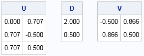
Notice that, to save memory, only the diagonal elements of the matrix Σ are returned in the vector D. You can explicitly form Σ = diag(D) if desired. Geometrically, the linear transformation that corresponds to V rotates a vector in the domain by about 30 degrees, the matrix D scales it by 2 and 0.5 in the coordinate directions, and U inserts it into a three-dimensional space, and applies another rotation.
My next blog post shows how the SVD enables you to reduce the dimension of a data matrix by using a low-rank approximation, which has applications to image compression and de-noising.

8 Comments
Fantastic explanation! This is the first time I feel like I understand what the svd is actually doing.
Thanks, Rick. The SVD is also the brains behind the Belsley-Kuh-Welsch collinearity diagnostics in PROC REG.
Good to hear from you, Charlie. You are mathematically correct. Numerically, PROC REG uses the eigenvalue decomposition of the symmetric covariance or correlation matrix (as stated in the documentation), which is more efficient. You can derive the spectral (eigenvalue) decomposition from the SVD:
If X = UDV` then
X`X = VD`U`UDV`
= VD`DV` by orthogonality
= VQV` where Q=D*D is the matrix of eigenvalues.
That proves the spectral decomposition. Because PROC REG has to compute the X`X matrix for regression, it uses that matrix for the collinearity diagnostics, too.
1976 Matrix Singular Value Decomposition Film at the Los Alamos National Laboratory
https://www.youtube.com/watch?v=R9UoFyqJca8
Hi Rick,
Regarding this statement:" The principal components of A.T * A are the columns of the V matrix; the scores are the columns of U":
1) Sometimes I'm very confused by the terminologies used by different authors. “principal components” and “scores” in this blog can be read as “principal axes/principal directions” and “principal components” respectively in other literature.
2) The V in A = U Σ V.T, is computed as the eigenvectors of A.T * A. so, the phrase “The principal components of A.T * A” might not be appropriate, since it is the principal components (or principal axes) for the data A itself.
3) The scores (or principal components used by other authors) are not the columns of U; they are columns of U * Σ or A*V if my memory serves me well …
Thanks for writing. Yes, the terminology is difficult to follow between different authors. I tried to be consistent with SAS documentation and with J. E. Jackson's comprehensive User's Guide to Principal Components, which I consider to be one of the best books on PCA.
In statistics, the word "scores" seems to mean "coefficients that enable you to write one set of variables as a linear combination of a set of basis vectors." Thus "scores" don't have an exact meaning until you specify an exact basis. If you choose V.T for the (orthonormal) basis, then the "scores for A" are U*Sigma, as you say in (3). However, if you choose Sigma.V.T as a basis, then the "scores for A" are just U. Some authors call Sigma*V.T the principal components; others use V.T, which are also called the principal component directions.
I have read lot of articles and none of them explained it's geometrical interpretation so clearly. Thank-you very much for this article.
Pingback: What are biplots? - The DO Loop