Recently, I was asked whether SAS can perform a principal component analysis (PCA) that is robust to the presence of outliers in the data. A PCA requires a data matrix, an estimate for the center of the data, and an estimate for the variance/covariance of the variables. Classically, these estimates are the mean and the Pearson covariance matrix, respectively, but if you replace the classical estimates by robust estimates, you can obtain a robust PCA.
This article shows how to implement a classical (non-robust) PCA by using the SAS/IML language and how to modify that classical analysis to create a robust PCA.
A classical principal component analysis in SAS
The PRINCOMP procedure in SAS computes a classical principal component analysis. You can analyze the correlation matrix (the default) or the covariance matrix of the variables (the COV option). You can create scree plots, pattern plots, and score plots automatically by using ODS graphics. If you want to apply rotations to the factor loadings, you can use the FACTOR procedure.
Let's use PROC PRINCOMP perform a simple PCA. The PROC PRINCOMP results will be the basis of comparison when we implement the PCA in PROC IML. The following example is taken from the Getting Started example in the PROC PRINCOMP documentation. The procedure analyzes seven crime rates for the 50 US states in 1977, based on the correlation matrix. (The documentation provides the data.)
proc princomp data=Crime /* add COV option for covariance analysis */ outstat=PCAStats_CORR out=Components_CORR plots=score(ncomp=4); var Murder Rape Robbery Assault Burglary Larceny Auto_Theft; id State; ods select Eigenvectors ScreePlot '2 by 1' '4 by 3'; run; proc print data=Components_CORR(obs=5); var Prin:; run; |
To save space, the output from PROC PRINCOMP is not shown, but it includes a table of the eigenvalues and principal component vectors (eigenvectors) of the correlation matrix, as well as a plot of the scores of the observations, which are the projection of the observations onto the principal components. The procedure writes two data sets: the eigenvalues and principal components are contained in the PCAStats_CORR data set and the scores are contained in the Components_CORR data set.
A classical principal component analysis in SAS/IML
Assume that the data consists of n observations and p variables and assume all values are nonmissing. If you are comfortable with multivariate analysis, a principal component analysis is straightforward: the principal components are the eigenvectors of a covariance or correlation matrix, and the scores are the projection of the centered data onto the eigenvector basis. However, if it has been a few years since you studied PCA, Abdi and Williams (2010) provides a nice overview of the mathematics. The following matrix computations implement the classical PCA in the SAS/IML language:
proc iml; reset EIGEN93; /* use "9.3" algorithm, not vendor BLAS (SAS 9.4m3) */ varNames = {"Murder" "Rape" "Robbery" "Assault" "Burglary" "Larceny" "Auto_Theft"}; use Crime; read all var varNames into X; /* X = data matrix (assume nonmissing) */ close; S = cov(X); /* estimate of covariance matrix */ R = cov2corr(S); /* = corr(X) */ call eigen(D, V, R); /* D=eigenvalues; columns of V are PCs */ scale = T( sqrt(vecdiag(S)) ); /* = std(X) */ B = (X - mean(X)) / scale; /* center and scale data about the mean */ scores = B * V; /* project standardized data onto the PCs */ print V[r=varNames c=("Prin1":"Prin7") L="Eigenvectors"]; print (scores[1:5,])[c=("Prin1":"Prin7") format=8.5 L="Scores"]; |
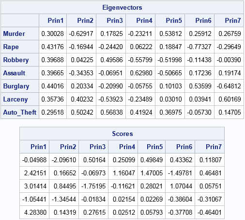
The principal components (eigenvectors) and scores for these data are identical to the same quantities that were produced by PROC PRINCOMP. In the preceding program I could have directly computed R = corr(X) and scale = std(X), but I generated those quantities from the covariance matrix because that is the approach used in the next section, which computes a robust PCA.
If you want to compute the PCA from the covariance matrix, you would use S in the EIGEN call, and define B = X - mean(X) as the centered (but not scaled) data matrix.
A robust principal component analysis
This section is based on a similar robust PCA computation in Wicklin (2010). The main idea behind a robust PCA is that if there are outliers in the data, the covariance matrix will be unduly influenced by those observations. Therefore you should use a robust estimate of the covariance matrix for the eigenvector computation. Also, the arithmetic mean is unduly influenced by the outliers, so you should center the data by using a robust estimate of center before you form the scores.
SAS/IML software provides the MCD subroutine for computing robust covariance matrices and robust estimates of location. If you replace the COV and MEAN functions in the previous section by a call to the MCD subroutine, you obtain a robust PCA, as follows:
/* get robust estimates of location and covariance */ N = nrow(X); p = ncol(X); /* number of obs and variables */ optn = j(8,1,.); /* default options for MCD */ optn[4]= floor(0.75*N); /* override default: use 75% of data for robust estimates */ call MCD(rc,est,dist,optn,x); /* compute robust estimates */ RobCov = est[3:2+p, ]; /* robust estimate of covariance */ RobLoc = est[1, ]; /* robust estimate of location */ /* use robust estimates to perform PCA */ RobCorr = cov2corr(RobCov); /* robust correlation */ call eigen(D, V, RobCorr); /* D=eigenvalues; columns of V are PCs */ RobScale = T( sqrt(vecdiag(RobCov)) ); /* robust estimates of scale */ B = (x-RobLoc) / RobScale; /* center and scale data */ scores = B * V; /* project standardized data onto the PCs */ |
Notice that the SAS/IML code for the robust PCA is very similar to the classical PCA. The only difference is that the robust estimates of covariance and location (from the MCD call) are used instead of the classical estimates.
If you want to compute the robust PCA from the covariance matrix, you would use RobCov in the EIGEN call, and define B = X - RobLoc as the centered (but not scaled) data matrix.
Comparing the classical and robust PCA
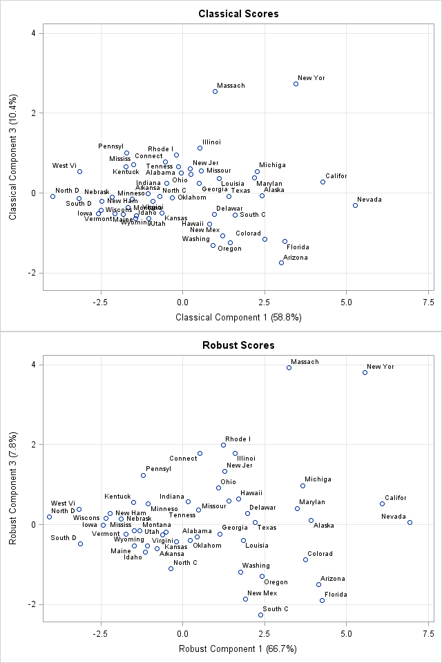
You can create a score plot to compare the classical scores to the robust scores. The Getting Started example in the PROC PRINCOMP documentation shows the classical scores for the first three components. The documentation suggests that Nevada, Massachusetts, and New York could be outliers for the crime data.
You can write the robust scores to a SAS data set and used the SGPLOT procedure to plot the scores of the classical and robust PCA on the same scale. The first and third component scores are shown to the right, with abbreviated state names serving as labels for the markers. (Click to enlarge.) You can see that the robust first-component scores for California and Nevada are separated from the other states, which makes them outliers in that dimension. (The first principal component measures overall crime rate.) The robust third-component scores for New York and Massachusetts are also well-separated and are outliers for the third component. (The third principal component appears to contrast murder with rape and auto theft with other theft.)
Because the crime data does not have huge outliers, the robust PCA is a perturbation of the classical PCA, which makes it possible to compare the analyses. For data that have extreme outliers, the robust analysis might not resemble its classical counterpart.
If you run an analysis like this on your own data, remember that eigenvectors are not unique and so there is no guarantee that the eigenvectors for the robust correlation matrix will be geometrically aligned with the eigenvectors from the classical correlation matrix. For these data, I multiplied the second and fourth robust components by -1 because that seems to make the score plots easier to compare.
Summary
In summary, you can implement a robust principal component analysis by using robust estimates for the correlation (or covariance) matrix and for the "center" of the data. The MCD subroutine in SAS/IML language is one way to compute a robust estimate of the covariance and location of multivariate data. The SAS/IML language also provides ways to compute eigenvectors (principal components) and project the (centered and scaled) data onto the principal components.
You can download the SAS program that computes the analysis and creates the graphs.
As discussed in Hubert, Rousseeuw, and Branden (2005), the MCD algorithm is most useful for 100 or fewer variables. They describe an alternative computation that can support a robust PCA in higher dimensions.
References
- Abdi and Williams (2010) "Principal component analysis," WIREs Computational Statistics, p 433–459.
- Hubert, Rousseeuw, and Branden (2005) "ROBPCA: A New Approach to Robust PrincipalComponent Analysis," Technometrics.
- Wicklin (2010) "Rediscovering SAS/IML Software: Modern Data Analysis for the Practicing Statistician." Robust PCA on p. 9–11.

10 Comments
Hi Rick, This is an interesting post. Is the robust covariance matrix guaranteed to be nonnegative definite? It occurred to me that you might want to use PROC IML to compute the robust covariance matrix and then put it back into PROC PRINCOMP in a TYPE=COV data set for the final PCA. I suppose the answer to my question does not matter from a certain point of view. PROC PRINCOMP requires symmetry in the covariance part of the TYPE=COV data set, but it does not require the matrix to be nonnegative definite. It still runs fine when it encounters negative eigenvalues. Still, if I were to use this technique, I would want to know more about the robust covariance matrix. Does it match the covariance matrix of a set of transformed variables?
Regarding the robust covariance matrix, the MCD algorithm randomly chooses K observations, computes the covariance matrix for those points, repeats the process many times, and returns the covariance matrix that has the smallest determinant. (In the example, K is 75% of the total observations.) Thus the robust matrix is a REAL covariance matrix, and consequently is always positive semidefinite.
Your idea about using a TYPE=COV data set is excellent. You could write the matrix from IML and then input it as a type=COV data set. You could then get the eigenvectors/PCs and scree plots. You would use PROC SCORE to get the PC scores, which has the advantage that PROC SCORE handles missing values. The following SAS calls give the general idea:
Rick,
Great idea.
SAS should integrate this robust PCA into PROC PRINCOMP .
Thank you for this information. Is there any way to incorporate pre-specified weights into the robust estimates?
That's an interesting question. I assume that you mean a weight for each observation. I believe the answer is yes. You can take your data matrix, X, and multiply each row by the square root of the weight for that row. If you call the new matrix Y, then Y=sqrt(w)#X. The classical covariance matrix for Y is therefore proportional to X`*W*X, which is the classical weighted scatter matrix. The MCD matrix will be a robust weighted covariance estimate. I haven't actually done it, but this method seems valid.
HOW CAN I WRITE RPCA IN SPSS LANGUAGE
I DON'T KNOW. ASK AT AN SPSS DISCUSSION FORUM.
When implementing the robust PCA, should the resulting factor scores still be uncorrelated? Implementing the classical PCA code generates scores with a diagonal covariance matrix, where the diagonal elements are equal to the corresponding eigenvalues. However, when I implement the robust PCA, the covariance matrix for the scores is no longer diagonal, and the diagonal elements are no longer the corresponding eigenvalues. How can I use the robust PCA to generate uncorrelated factor scores?
Thanks for your help!
You are correct. The classical PCA generates scores with diagonal covariance because the data are standardized by (X - mean(X))/ std(X) and cov(X) is used for the eigen decomposition. In robust PCA, the data are not centered and scaled in the same way. Therefore the classical geometry is distorted. in the robust PCA, you should not expect the CLASSICAL covariance of the robust scores to be diagonal; you expect the ROBUST covariance of the scores to be diagonal.
That makes sense, thanks very much for your response. I was able to verify this using my data; the robust covariance of the scores was indeed diagonal.