Skewness is a measure of the asymmetry of a univariate distribution. I have previously shown how to compute the skewness for data distributions in SAS. The previous article computes Pearson's definition of skewness, which is based on the standardized third central moment of the data.
Moment-based statistics are sensitive to extreme outliers. A single extreme observation can radically change the mean, standard deviation, and skewness of data. It is not surprising, therefore, that there are alternative definitions of skewness. One robust definition of skewness that is intuitive and easy to compute is a quantile definition, which is also known as the Bowley skewness or Galton skewness.
A quantile definition of skewness
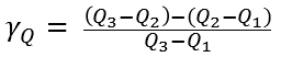
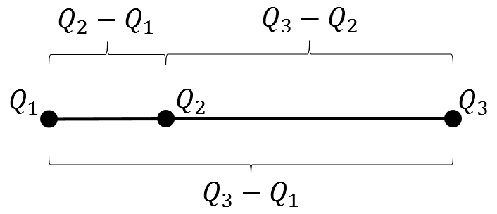
The quantile definition of skewness uses Q1 (the lower quartile value), Q2 (the median value), and Q3 (the upper quartile value). You can measure skewness as the difference between the lengths of the upper quartile (Q3-Q2) and the lower quartile (Q2-Q1), normalized by the length of the interquartile range (Q3-Q1). In symbols, the quantile skewness γQ is
You can visualize this definition by using the figure to the right.
 For a symmetric distribution, the quantile skewness is 0 because the length Q3-Q2 is equal to the length Q2-Q1.
If the right length (Q3-Q2) is larger than the left length (Q2-Q1), then the quantile skewness is positive.
If the left length is larger, then the quantile skewness is negative.
For the extreme cases when Q1=Q2 or Q2=Q3, the quantile skewness is ±1.
Consequently, whereas the Pearson skewness can be any real value, the quantile skewness is bounded in the interval [-1, 1].
The quantile skewness is not defined if Q1=Q3, just as the Pearson skewness is not defined when the variance of the data is 0.
For a symmetric distribution, the quantile skewness is 0 because the length Q3-Q2 is equal to the length Q2-Q1.
If the right length (Q3-Q2) is larger than the left length (Q2-Q1), then the quantile skewness is positive.
If the left length is larger, then the quantile skewness is negative.
For the extreme cases when Q1=Q2 or Q2=Q3, the quantile skewness is ±1.
Consequently, whereas the Pearson skewness can be any real value, the quantile skewness is bounded in the interval [-1, 1].
The quantile skewness is not defined if Q1=Q3, just as the Pearson skewness is not defined when the variance of the data is 0.
There is an intuitive interpretation for the quantile skewness formula. Recall that the relative difference between two quantities R and L can be defined as their difference divided by their average value. In symbols, RelDiff = (R - L) / ((R+L)/2). If you choose R to be the length Q3-Q2 and L to be the length Q2-Q1, then quantile skewness is half the relative difference between the lengths.
Compute the quantile skewness in SAS
It is instructive to simulate some skewed data and compute the two measures of skewness. The following SAS/IML statements simulate 1000 observations from a Gamma(a=4) distribution. The Pearson skewness of a Gamma(a) distribution is 2/sqrt(a), so the Pearson skewness for a Gamma(4) distribution is 1. For a large sample, the sample skewness should be close to the theoretical value. The QNTL call computes the quantiles of a sample.
/* compute the quantile skewness for data */ proc iml; call randseed(12345); x = j(1000, 1); call randgen(x, "Gamma", 4); skewPearson = skewness(x); /* Pearson skewness */ call qntl(q, x, {0.25 0.5 0.75}); /* sample quartiles */ skewQuantile = (q[3] -2*q[2] + q[1]) / (q[3] - q[1]); print skewPearson skewQuantile; |
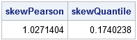
For this sample, the Pearson skewness is 1.03 and the quantile skewness is 0.174. If you generate a different random sample from the same Gamma(4) distribution, the statistics will change slightly.
Relationship between quantile skewness and Pearson skewness
In general, there is no simple relationship between quantile skewness and Pearson skewness for a data distribution. (This is not surprising: there is also no simple relationship between a median and a mean, nor between the interquartile range and the standard deviation.) Nevertheless, it is interesting to compare the Pearson skewness to the quantile skewness for a particular probability distribution.
For many probability distributions, the Pearson skewness is a function of the parameters of the distribution. To compute the quantile skewness for a probability distribution, you can use the quantiles for the distribution. The following SAS/IML statements compute the skewness for the Gamma(a) distribution for varying values of a.
/* For Gamma(a), the Pearson skewness is skewP = 2 / sqrt(a). Use the QUANTILE function to compute the quantile skewness for the distribution. */ skewP = do(0.02, 10, 0.02); /* Pearson skewness for distribution */ a = 4 / skewP##2; /* invert skewness formula for the Gamma(a) distribution */ skewQ = j(1, ncol(skewP)); /* allocate vector for results */ do i = 1 to ncol(skewP); Q1 = quantile("Gamma", 0.25, a[i]); Q2 = quantile("Gamma", 0.50, a[i]); Q3 = quantile("Gamma", 0.75, a[i]); skewQ[i] = (Q3 -2*Q2 + Q1) / (Q3 - Q1); /* quantile skewness for distribution */ end; title "Pearson vs. Quantile Skewness"; title2 "Gamma(a) Distributions"; call series(skewP, skewQ) grid={x y} label={"Pearson Skewness" "Quantile Skewness"}; |
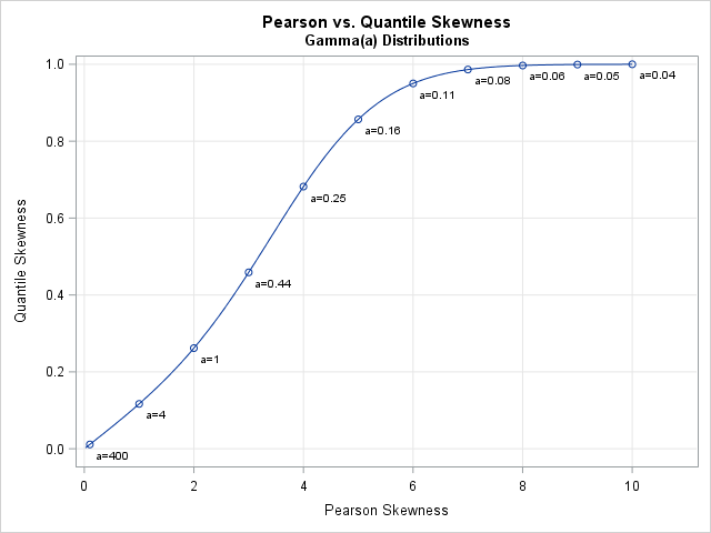
The graph shows a nonlinear relationship between the two skewness measures. This graph is for the Gamma distribution; other distributions would have a different shape. If a distribution has a parameter value for which the distribution is symmetric, then the graph will go through the point (0,0). For highly skewed distributions, the quantile skewness will approach ±1 as the Pearson skewness approaches ±∞.
Alternative quantile definitions
Several researchers have noted that there is nothing special about using the first and third quartiles to measure skewness. An alternative formula (sometimes called Kelly's coefficient of skewness) is to use deciles: γKelly = ((P90 - P50) - (P50 - P10)) / (P90 - P10). Hinkley (1975) considered the q_th and (1-q)_th quantiles for arbitrary values of q.
Conclusions
The quantile definition of skewness is easy to compute. In fact, you can compute the statistic by hand without a calculator for small data sets. Consequently, the quantile definition provides an easy way to quickly estimate the skewness of data. Since the definition uses only quantiles, the quantile skewness is robust to extreme outliers.
At the same time, the Bowley-Galton quantile definition has several disadvantages. It uses only the central 50% of the data to estimate the skewness. Two different data sets that have the same quartile statistics will have the same quantile skewness, regardless of the shape of the tails of the distribution. And, as mentioned previously, the use of the 25th and 75th percentiles are somewhat arbitrary.
Although the Pearson skewness is widely used in the statistical community, it is worth mentioning that the quantile definition is ideal for use with a box-and-whisker plot. The Q1, Q2, and Q2 quartiles are part of every box plot. Therefore you can visually estimate the quantile skewness as the relative difference between the lengths of the upper and lower boxes.

1 Comment
Does quantile skewness differ much from medcouple?