A reader commented on last week's article about constructing symmetric intervals. He wanted to know if I created it in SAS.
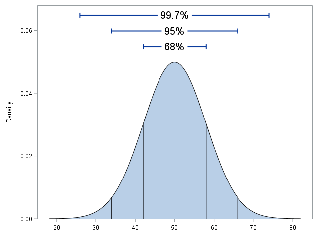
Yes, the graph, which illustrates the so-called 68-95-99.7 rule for the normal distribution, was created by using several statements in the SGPLOT procedure in Base SAS
- The SERIES statement creates the bell-shaped curve.
- The BAND statement creates the shaded region under the curve.
- The DROPLINE statement creates the vertical lines from the curve to the X axis.
- The HIGHLOW statement creates the horizontal lines that indicate interval widths.
- The TEXT statement creates the text labels "68%", "95%", and "99.7%".
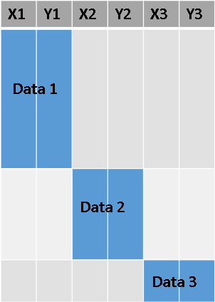
If you follow some simple rules, it is easy to use PROC SGPLOT the overlay multiple curves and lines on a graph. The key is to organize the underlying data into a block form, as shown conceptually in the plot to the right. I use different variable names for each component of the plot, and I set the values of the other variables to missing when they are no longer relevant. Each statement uses only the variables that are relevant for that overlay.
The following DATA step creates the data for the 68-95-99.7 graph. Can you match up each section with the SGPLOT statements that overlay various components to create the final image?
data NormalPDF; mu = 50; sigma = 8; /* parameters for the normal distribution N(mu, sigma) */ /* 1. Data for the SERIES and BAND statements */ do m = -4 to 4 by 0.05; /* x in [mu-4*sigma, mu+4*sigma] */ x = mu + m*sigma; f = pdf("Normal", x, mu, sigma); /* height of normal curve */ output; end; x=.; f=.; /* 2. Data for vertical lines at mu + m *sigma, m=-3, -2, -1, 1, 2, 3 */ do m =-3 to 3; if m=0 then continue; /* skip m=0 */ Lx = mu + m*sigma; /* horiz location of segment */ Lf = pdf("Normal", Lx, mu, sigma); /* vertical height of segment */ output; end; LX = .; Lf = .; /* 3. Data for horizontal lines. Heights are 1.1, 1.2, and 1.3 times the max height of the curve */ Tx = mu; /* text centered at mu */ fMax = pdf("Normal", mu, mu, sigma); /* highest point of curve */ Text = "68% "; /* 68% interval */ TL = mu - sigma; TR = mu + sigma; /* Left/Right endpoints of interval */ Ty = 1.1 * fMax; /* height of label and segment */ output; Text = "95% "; /* 95% interval */ TL = mu - 2*sigma; TR = mu + 2*sigma; /* Left/Right endpoints of interval */ Ty = 1.2 * fMax; /* height of label and segment */ output; Text = "99.7%"; /* 99.7% interval */ TL = mu - 3*sigma; TR = mu + 3*sigma; /* Left/Right endpoints of interval */ Ty = 1.3 * fMax; /* height of label and segment */ output; keep x f Lx Lf Tx Ty TL TR Text; run; proc sgplot data=NormalPDF noautolegend; band x=x upper=f lower=0; series x=x y=f / lineattrs=(color=black); dropline x=Lx y=Lf / dropto=x lineattrs=(color=black); highlow y=Ty low=TL high=TR / lowcap=serif highcap=serif lineattrs=(thickness=2); text x=Tx y=Ty text=Text / backfill fillattrs=(color=white) textattrs=(size=14); yaxis offsetmin=0 min=0 label="Density"; xaxis values=(20 to 80 by 10) display=(nolabel); run; |

8 Comments
Rick,
Title should be 68-95-99.7 rule ?
Yes! Not sure how "97.5" got in there...thanks!
Rick,
I think every statistical guy would get this kind of thing. 1.96 --> 0.975
This looks like a great graphic, which I would like to modify to illustrate how to calculate one and two sided p-values. Unfortunately, neither "dropline" nor "text" statements work for me in 9.4 (TS1M0). Can you suggest a work-around?
See the article "Create a density curve with shaded tails."
Use the SCATTER statement with the MARKERCHAR= option to plot text instead of markers. If you have questions, ask at the SAS Graphics Support Community.
See the article "Create a density curve with shaded tails."
Use the SCATTER statement with the MARKERCHAR= option to plot text instead of markers. If you have questions, ask at the SAS Graphics Support Community.
Pingback: Extreme values: What is an extreme value for normally distributed data? - The DO Loop
Pingback: The math you learned in school: Yes, it’s useful! - The DO Loop