The article uses the SAS DATA step and Base SAS procedures to estimate the coverage probability of the confidence interval for the mean of normally distributed data. This discussion is based on Section 5.2 (p. 74–77) of Simulating Data with SAS.
What is a confidence interval?
Recall that a confidence interval (CI) is an interval estimate that potentially contains the population parameter. Because the CI is an estimate, it is computed from a sample. A confidence interval for a parameter is derived by knowing (or approximating) the sampling distribution of a statistic. For symmetric sampling distributions, the CI often has the form m ± w(α, n), where m is an unbiased estimate of the parameter and w(α, n) is a width that depends on the significance level α, the sample size n, and the standard error of the estimate.
Due to sampling variation, the confidence interval for a particular sample might not contain the parameter. A 95% confidence interval means that if you collect a large number of samples and construct the corresponding confidence intervals, then about 95% of the intervals will contain (or "cover") the parameter.
For example, a well-known formula is the confidence interval of the mean. If the population is normally distributed, then a 95% confidence interval for the population mean, computed from a sample of size n, is
[ xbar – tc s / sqrt(n),
xbar + tc s / sqrt(n) ]
where
- xbar is the sample mean
- tc = t1-α/2, n-1 is the critical value of the t statistic with significance α and n-1 degrees of freedom
- s / sqrt(n) is the standard error of the mean, where s is the sample standard deviation.
Coverage probability
The preceding discussion leads to the simulation method for estimating the coverage probability of a confidence interval. The simulation method has three steps:
- Simulate many samples of size n from the population.
- Compute the confidence interval for each sample.
- Compute the proportion of samples for which the (known) population parameter is contained in the confidence interval. That proportion is an estimate for the empirical coverage probability for the CI.
You might wonder why this is necessary. Isn't the coverage probability always (1-α) = 0.95? No, that is only true when the population is normally distributed (which is never true in practice) or the sample sizes are large enough that you can invoke the Central Limit Theorem. Simulation enables you to estimate the coverage probability for small samples when the population is not normal. You can simulate from skewed or heavy-tailed distributions to see how skewness and kurtosis affect the coverage probability. (See Chapter 16 of Simulating Data with SAS.)
The simulation method for estimating coverage probability
Let's use simulation to verify that the formula for a CI of the mean is valid when you draw samples from a standard normal population. The following DATA step simulates 10,000 samples of size n=50:
%let N = 50; /* size of each sample */ %let NumSamples = 10000; /* number of samples */ /* 1. Simulate samples from N(0,1) */ data Normal(keep=SampleID x); call streaminit(123); do SampleID = 1 to &NumSamples; /* simulation loop */ do i = 1 to &N; /* N obs in each sample */ x = rand("Normal"); /* x ~ N(0,1) */ output; end; end; run; |
The second step is to compute the confidence interval for each sample. You can use PROC MEANS to compute the confidence limits. The LCLM= and UCLM= outputs the lower and upper endpoints of the confidence interval to a SAS data set. I also output the sample mean for each sample. Notice that the BY statement is an efficient way to analyze all samples in a simulation study.
/* 2. Compute statistics for each sample */ proc means data=Normal noprint; by SampleID; var x; output out=OutStats mean=SampleMean lclm=Lower uclm=Upper; run; |
The third step is to count the proportion of samples for which the confidence interval contains the value of the parameter. For this simulation study, the value of the population mean is 0. The following DATA step creates an indicator variable that has the value 1 if 0 is within the confidence interval for a sample, and 0 otherwise. You can then use PROC FREQ to compute the proportion of intervals that contain the mean. This is the empirical coverage probability. If you want to get fancy, you can even use the BINOMIAL option to compute a confidence interval for the proportion.
/* 3a. How many CIs include parameter? */ data OutStats; set OutStats; label ParamInCI = "Parameter in CI"; ParamInCI = (Lower<0 & Upper>0); /* indicator variable */ run; /* 3b. Nominal coverage probability is 95%. Estimate true coverage. */ proc freq data=OutStats; tables ParamInCI / nocum binomial(level='1' p=0.95); run; |
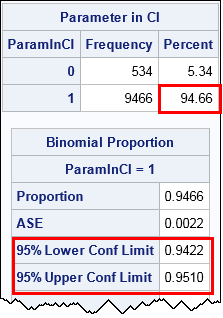
The output from PROC FREQ tells you that the empirical coverage (based on 10,000 samples) is 94.66%, which is very close to the theoretical value of 95%. The output from the BINOMIAL option estimates that the true coverage is in the interval [0.9422,0.951], which includes 0.95. Thus the simulation supports the assertion that the standard CI of the mean has 95% coverage when a sample is drawn from a normal population.
Visualizing the simulation study
You can draw a graph that shows how the confidence intervals depend on the random samples. The following graph shows the confidence intervals for 100 samples. The center of each CI is the sample mean.
proc format; /* display 0/1 as "No"/"Yes" */ value YorN 0="No" 1="Yes"; run; ods graphics / width=6.5in height=4in; proc sgplot data=OutStats(obs=100); format ParamInCI YorN.; title "95% Confidence Intervals for the Mean"; title2 "Normal Data"; scatter x=SampleID y=SampleMean / group=ParamInCI markerattrs=(symbol=CircleFilled); highlow x=SampleID low=Lower high=Upper / group=ParamInCI legendlabel="95% CI"; refline 0 / axis=y; yaxis display=(nolabel); run; |
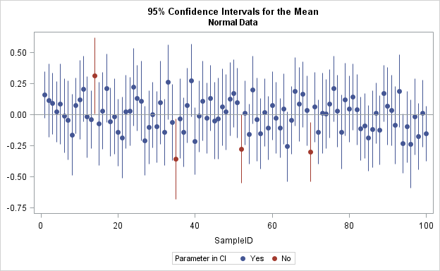
The reference line shows the mean of the population. Samples for which the population mean is inside the confidence interval are shown in blue. Samples for which the population mean is not inside the confidence interval are shown in red.
You can see how sample variability affects the confidence intervals. In four random samples (shown in red) the values in the sample are so extreme that the confidence interval does not include the population mean. Thus the estimate of the coverage probability is 96/100 = 96% for these 100 samples. This graph shows why the term "coverage probability" is used: it is the probability that one of the vertical lines in the graph will "cover" the population mean.
The coverage probability for nonnormal data
The previous simulation confirms that the empirical coverage probability of the CI is 95% for normally distributed data. You can use simulation to understand how that probability changes if you sample from nonnormal data. For example, in the DATA step that simulates the samples, replace the call to the RAND function with the following line:
x = rand("Expo") - 1; /* x + 1 ~ Exp(1) */ |
You can then rerun the simulation study. This time the samples are drawn from a (shifted) exponential distribution that has mean 0 and unit variance. The skewness for this distribution is 2 and the excess kurtosis is 6. The result from PROC FREQ is that only about 93.5% of the confidence intervals (using the standard formula) cover the true population mean. Consequently, the formula for the CI, which has 95% coverage for normal data, only has about 93.5% coverage for this exponential data.
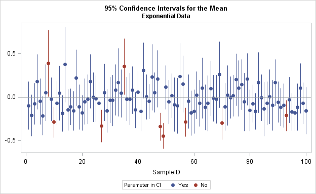
You can create a graph that visualizes the confidence intervals for the exponential data. Again, only the first 100 samples are shown. In this graph, the CIs for nine samples do not contain the population mean, which implies a 91% empirical coverage.
You can also write a SAS/IML program. An example of using SAS/IML to estimate the coverage probability of a confidence interval is posted on the SAS/IML File Exchange.
In summary, you can use simulation to estimate the empirical coverage probability for a confidence interval. In many cases the formula for a CI is based on an assumption about the population distribution, which determines the sampling distribution of the statistic. Simulation enables you to explore how the coverage probability changes when the population does not satisfy the theoretical assumptions.

50 Comments
So I'm sure I understand, you said: "Because the CI is an estimate, it is computed from a sample." Is this the same thing as saying, "Because the CI is computed from a sample, it is an estimate?"
Yes, that is what I meant. I think I phrased it that way to emphasize that a CI is not composed of population parameters (mu and sigma), it is formed from sample statistics.
I need assistance on how to calculate coverage probability for each model parameters (e.g beta1, beta2 etc)
Most SAS regression procedures have an option on the MODEL statement that you can use to get CIs for the parameters. See the doc. For example:
PROC REG; MODEL Y = X / CLB; RUN;
PROC GLM; MODEL Y = X / CLPARM; RUN;
PROC GENMOD; MODEL Y = X / LRCI WALDCI; RUN;
etc.
The SAS code did not give 95% coverage probability for each model parameter. I want 95% coverage probability for beta0, beta1, beta2 etc.
I suggest you post sample data and the SAS code that you are using the SAS Statistical Procedures Community. That is the best way to ask questions about SAS procedures.
Pingback: Simultaneous confidence intervals for a multivariate mean - The DO Loop
Hi Dr. Rick Wicklin, what is the recommended number of samples for coverage probability of the confidence interval for parameter of the model. Thank you.
In my book Simulating Data with SAS (2013, p. 96) I say, "that is a difficult question to answer. The number of samples that you need depends on characteristics of the sampling distribution. Lower order moments of the sampling distribution (such as the mean) require fewer samples than statistics that are functions of higher order moments, such as the variance and skewness. You might need many, many, samples to capture the extreme tail behavior of a sampling distribution. A popular choice in research studies is 10,000 or more samples. However, do not be a slave to any particular number. The best approach is to understand what you are trying to estimate and to report not only point estimates but also standard errors and/or confidence intervals."
Thank you for the reply.
Hello,
how can I calculate the Probability, having Z calculated? I can't use tables as far as I'm getting Z(Confidence Intervals) from SQL querry.
Are you asking how to compute the probability for a given critical value of a distribution? Use the CDF function.
Pingback: A simple trick to construct symmetric intervals - The DO Loop
Hi,
Suppose I simulate 1000 times and i get a coverage proportion of say 94%: how do I know what the acceptable level of variation about 95% is please?
re-read the section that mentions PROC FREQ and the BINOMIAL option. If the estimate is p=0.94, then there were 940 "successes" in 1000 "trials." The estimate is a binomial proportion, so an estimate for the variance is p*(1-p)/n = (0.94)(0.06)/1000 = 5.64E-5.
How do I calculate coverage probability for a nonparametric estimator of a finite population total using the edgeworth functions? particularly in R?
I suggest you ask questions like this on a public discussion forum such as Stack Overflow.
This is great!! What changes would I have to make in the code above to apply this to a population proportion (rather than mean)? I'm rather new to SAS and am having some difficulty. Thanks!
Since you are having problems, I advise you to post your problem (along with sample code) to one of the SAS Support Communities. For statistical questions and simulation studies, I recommend the SAS Statistical Procedures Community.
Thanks Rick for the informative discussions. I want to estimate coverage probability for treatment difference using lsmeans from sample distributions. The problem is, I don’t have define value of the difference (known parameter) that I can use to estimate the coverage proportion. How can I decide on this value?
I don't understand your question. You can only estimate a coverage proportion when you know the true value of the parameter. By definition, the coverage probability is the proportion of CIs (estimated from random samples) that include the parameter. In a simulation study, you always know the true parameter and the distribution of the population. Even when you estimate the CI for a contrast (difference) or a linear combination of the parameters, you know the true value.
Thanks Rick for your reply. To be more clear, I have simulated M=500 samples of size N=600 from a proposed linear mixed model using real life data from a study that was investigating effect of two treatments on blood pressure measures. I now want to compare my proposed statistical model with two other existing models using a set of performance measurements (e.g. MSE, Coverage probability,...etc). The investigators of the blood pressure study used a proposed effect size to compute the sample size. Is it sensible to assume the proposed effect size to be the true parameter, such that I can recode each of the computed lsmeans differences from the simulated M=500 samples, to 1 (if lsmeans differences>=effect size) and 0 (if lsmeans differences <effect size)?
It sounds like you used an estimate (beta) from a real study as the parameter for your simulation. That estimate is the best (hopefully, unbiased) estimate for the true parameter. The "assumed effect size" that determined the sample size is probably not a good estimate. It was based on a guess or on a small preliminary experiment. If you compare the MC estimates to the "assumed" effects, you will get biased results. I think you want to compare the MC estimates to beta. As far as the simulation is concerned, beta is the true parameter for the model.
Thank you very much Rick! This is very helpful.
Just to review the question, is it sensible to assume the proposed effect size to be the true parameter, such that I can estimate the lsmeans differences from the simulated M=500 samples and code each of the estimates with 95% confidence interval, to 1 if the 95% confidence interval of the lsmeans estimates for every sample includes the proposed effect size, or to 0 otherwise?
sir in a simple word we can say the coverage probability is defines as sum of the estimator each time fall in the interval than we divide the sum with total number of runs that we use for replication??is am getting right???
Yes. That is the definition of the empirical coverage probability in a simulation study.
Thank you for this informative article. Following from https://www.seku.ac.ke/
Thanks Rick for the informative discussions. I want to estimate coverage probability for treatment difference using lsmeans from sample distributions. The problem is, I don’t have define value of the difference (known parameter) that I can use to estimate the coverage proportion. How can I decide on this value?
In a simulation study, you always know the true value of parameters.
Hello Dr. Rick how can I calculate the CI for mean when X~N(Eta, Theta)? Could you please share the SAS code? Thanks.
What does coverage probability of one indicate?
It means that the parameter value is in 100% of the intervals.
can you give me usefulness of coverage probability with an example? how should i explain the usefulness?
Sure. See the Wikipedia article about coverage probability.
Pingback: What statistic should you use to display error bars for a mean? - The DO Loop
Hello Dr.Rick i run a simulation(using excel not familiar/no access to SAS) for finding the coverage probability of population mean a chi-squared distribution(degree of freedom 30) at 95%level based on normal distribution. My sample size are n=10, n=30 and n=50 for 200 confidence intervals. I found out my coverage probability is decreasing 97%, 95% and 92% as n increases from 10, 30 and 50. I believe this is because the confidence interval width is getting smaller so it is less likely to capture the parameter. However i thought that as we increase the sample size, the coverage should tends to the empherical 95% confidence interval. Please help on this(what might be the cause of the problem other than error on formulation). Thank you.
I don't know. Perhaps you are using a variance instead of a standard deviation? The mean of a chi-square distribution with k DOF is asymptotically distributed as N(nu=k, StdDev=sqrt(2*k/n)) as n->infinity. If you can't figure it out, I suggest you post the method and formulas that you are using to a statistics Q&A board, such as CrossValidated.
I just performed the simulation myself for k=30. When done correctly, the coverage probability is approximately 95% for all n>=10.
Ok, Thank you Dr. Rick, i might be making a wrong cross reference.
Pingback: Use simulations to evaluate the accuracy of asymptotic results - The DO Loop
Thanks Rick for the informative discussions. following from https://www.seku.ac.ke
please can someone help me with coverage probability r-codes of Wald Statistic and Peskun Statistic.
You can post your question and data to the SAS Support Communities: https://communities.sas.com/
Sir Kindly assist me to calculate the coverage probability for bootstrap C.I of regression coefficient in R.
Pingback: The distribution of the sample median - The DO Loop
What are some strategies one can employ to ensure accurate estimation of confidence intervals in simulation studies, considering the known true parameter values and population distribution