I saw an interesting mathematical result in Wired magazine. The original article was about mathematical research into prime numbers, but the article included the following tantalizing fact:
If Alice tosses a [fair]coin until she sees a head followed by a tail, and Bob tosses a coin until he sees two heads in a row, then on average, Alice will require four tosses while Bob will require six tosses (try this at home!), even though head-tail and head-head have an equal chance of appearing after two coin tosses.
Yes, I would classify that result as counter-intuitive! When I read this paragraph, I knew I had to simulate these coin tosses in SAS.
Why does head-tail happen sooner (on average)?
Define the "game" for Alice as a sequence of coin tosses that terminates in a head followed by a tail. For Bob, the game is a sequence of coin tosses that terminates in two consecutive heads.
You can see evidence that the result is true by looking at the possible sequence of tosses that end the game for Alice versus Bob. First consider the sequences for Alice that terminate with head-tail (HT). The following six sequences terminate in four or fewer tosses:
HT THT HHT THHT TTHT HHHT |
In contrast, among Bob's sequences that terminate with head-head (HH), only four require four or fewer tosses:
HH THH TTHH HTHH |
For Bob to "win" (that is, observe the sequence HH), he must first toss a head. On the next toss, if he obtains a head again, he wins. But if he observes a tail, he is must start over: He has to toss until a head appears, and the process continues.
In contrast, for Alice to "win" (that is, observe the sequence HT), she must first toss a head. If the next toss shows a tail, she wins. But if is a head, she doesn't start over. In fact, she is already halfway to winning on the subsequent toss.
This result is counterintuitive because a sequence is just as likely to terminate with HH as with HT. So Alice and Bob "win" equally often if they are observing flips of a single fair coin. However, the sequences for which Alice wins tend to be shorter than those for which Bob wins.
Counterintuitive property of coin tosses. Head-tail vs head-head #Statistics #Probability #Simulation Click To TweetA simulation of coin tosses
The following SAS DATA step simulates Alice and Bob tossing coins until they have each won 100,000 games. For each player, the program counts how many tosses are needed before the "winning" sequence occurs. A random Bernoulli number (0 or 1 with probability 0.5) simulates the coin toss.
data CoinFlip(keep= player toss); call streaminit(123456789); label Player = "Stopping Condition"; do i = 1 to 100000; do player = "HT", "HH"; /* first Alice tosses; then Bob */ first = rand("Bernoulli", 0.5); /* 0 is Tail; 1 is Head */ toss = 1; done = 0; do until (done); second = rand("Bernoulli", 0.5); toss = toss + 1; /* how many tosses until done? */ if player = "HT" then /* if Alice, ... */ done = (first=1 & second=0); /* stop when HT appears */ else /* if Bob, ... */ done = (first=1 & second=1); /* stop when HH appears */ first = second; /* remember for next toss */ end; output; end; end; run; proc means data=CoinFlip MAXDEC=1 mean median Q3 P90 max; class player; var toss; run; |
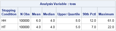
The MEANS procedure displays statistics about the length of each game. The mean (expected) length of the game for Bob (HH) is 6 tosses. 75% of games were resolved in eight tosses or less and 90% required 12 or less. In the 100,000 simulated games, the longest game that Bob played required 61 tosses before it terminated. (The maximum game length varies with the random number seed.)
In contrast, Alice resolved her 100,000 games by using about 50% fewer tosses. The mean (expected) length of the game for Alice (HT) is 4 tosses. 75% of the games required five or fewer tosses and 90% were completed in seven or fewer tosses. In the 100,000 simulated games, the longest game that Alice played required 22 tosses.
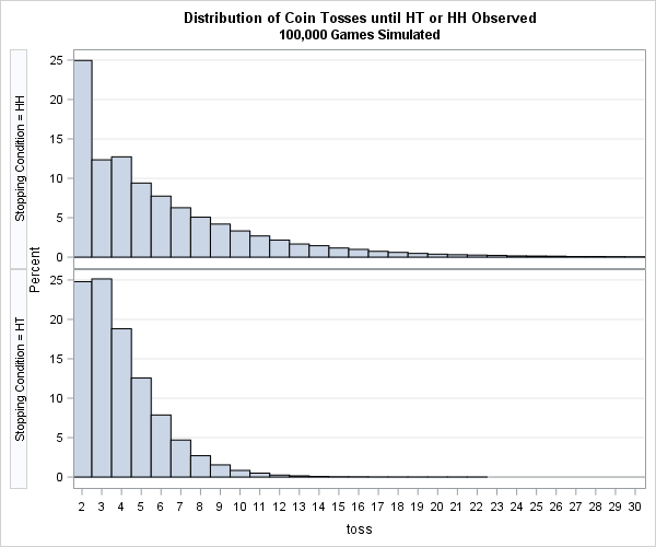
You can create a comparative histogram to compare the distribution of the game lengths. The distribution of the length of Bob's games is shown in the upper histogram. It has a long tail.
In contrast, the distribution of Alice's game lengths is shown in the bottom of the panel. The distribution drops off much more quickly than for Bob's games.
It is also enlightening to see the empirical cumulative distribution functions (ECDFs) for the number of tosses for each player. You can download a SAS program that creates the comparative histogram and the ECDFs. For skeptics, the program also contains a simulation that demonstrates that a sequence terminates with HH as often as it terminates with HT.
The result is not deep, but it reminds us that the human intuition gets confused by conditional probability. Like the classic the Monty Hall problem, simulation can convince us that a result is true, even when our intuition refuses to believe it.

12 Comments
Rick,
You didn't post the IML code yet ?
proc iml; toss=100000; x={H T}; current=sample(x,100//toss); next=current[,2:100]||repeat({' '},toss,1); ht=current+next; result=j(toss,2,.); do i=1 to toss; result[i,1]=min(loc(ht[i,]='HT'))+1; result[i,2]=min(loc(ht[i,]='HH'))+1; end; winner=choose(result[,1]>result[,2],'HH','HT'); create CoinFlip from result[c={'HT' 'HH'}]; append from result; close; create winner var{winner}; append; close; quit; proc means data=CoinFlip MAXDEC=1 n mean median Q3 P90 max ; run; proc sgplot data=CoinFlip; histogram HT/transparency=0.6 binwidth=1; histogram HH/transparency=0.6 binwidth=1; run; proc freq data=winner; tables winner / nocum binomial(level='HT'); run;Ah, this was a fun one to puzzle over. I have a programming background, so the differing state machines came to my mind in the shower.
I'm an R novice, so this is probably not the most elegant way to do this, but here's what I came up with:
SimFindMatch < - function (size, match, p = .5, sim = NULL, debug = FALSE) { # Generate size number of coin flips. if (is.null (sim)) { sim <- rbinom (size, 1, p) } if (debug) { print(sim) } # Loop through the results to see how soon the match occurs. found <- FALSE resetJ <- FALSE # i is the index into sim vector i <- 1 while ((i <= size) && !(found)) { endI <- i + length(match) - 1 if (debug) { print (cat ("sim[", i, "]:", sim[i], "endI:", endI, "\n")) } # If all elements in match[] do match where we are in sim, then we have a match! if (all (match == sim[i:endI])) { found = TRUE break } i <- i + 1 } if (found) return (i) else return (NULL) } SimMatches <- function (size, match, p = .5, n = 1000) { results <- vector (length = n) i <- 0 while (i < n) { results[i] = SimFindMatch (size, match, p) i <- i + 1 } return (results) } SimHeadsHeadsHeadsTails <- function (size, p = .5, n = 10000) { hhResults <- SimMatches (size, c (1,1), p, n) htResults <- SimMatches (size, c (1,0), p, n) breakMax <- max (hhResults, htResults) print (cat ("HH average:", mean (hhResults), " HT average:", mean (htResults), "\n")) # 1st plot in 1st row, 2nd in 2nd row layout(matrix(c(1,2), 2, 1, byrow = TRUE)) breaks <- seq (-5, breakMax +.5) hist (hhResults, breaks, main = "Distribution of Heads-Heads", xlab = "tosses", col = "lightgreen") hist (htResults, breaks, main = "Distribution of Heads-Tails", xlab = "tosses", col = "lightgreen") }Is this reasoning correct?
1. For the TH case, there is some number greater than or equal to zero of heads until the first tails, then some number greater than or equal to zero tails, until the next heads. That will be the first case of TH. The first number has a geometric distribution with parameter p=1/2, as does the second. So it's the sum of 2 r.v.s, each with mean 1/p=2 for a total of 4.
2. For the HH case, say there are some number of tails until the first heads. That would also be geometric. If the next toss is heads, it's done. That would be 1 + X where X has geometric distribution as above. But if the toss after heads turns up tails, then this needs to be repeated, until the toss after the heads is another heads. So it's like a random (geometric) number of these sequences, each of which is like 1 + X with X also geometric. So the expected number would be 2 * (2+1) = 2 * 3 = 6.
Looks fine. I like that you use the Geometric distribution.
Hi,
Very interesting, I also find for:
1/ HT, expectation of 4, with variance of 4 as well.
2/ HH, expectation of 6, with variance of 40, so 10 times higher than for HT.
2/ Sorry, variance is 22 for HH
Pingback: Markov transition matrices in SAS/IML - The DO Loop
I found this thread after watching TED talk by Peter Donnelly: How juries are fooled by statistics.
And I have this comment on your explanation in favor of Alice. You state that : "In contrast, for Alice to "win" (that is, observe the sequence HT), she must first toss a head. If the next toss shows a tail, she wins. But if is a head, she doesn't start over. In fact, she is already halfway to winning on the subsequent toss"
My conclusion is that if the first toss is H and the next one is again H, indeed she is already halfway, but Bob is DONE! He wins, the game end there. Or am i missing something?
Thnks for writing. You are correct that if you limit the game to two tosses, then each has an equal 25% chance of winning the game. However, if the game proceeds to three or more tosses, then Alice holds an advantage. For example, for exactly three tosses, Alice wins 2/8 times whereas Bob only wins 1/8 of the time.
But what happens if you make them compete against each other? For example, whoever has their sequence appear first wins.
I just ran this simulation and it's back to an equal 50/50 split. Alice loses her advantage (like @Eric said) because when Bob wins the HH she is no longer halfway to winning, Bob has already won.
Here is my Python code simulation for those interested:
import random
def flipcoin():
number = random.random()
if number > .5:
return 'H'
if number < .5:
return 'T'
if number == .5:
flipcoin()
def check_for_results(results):
if 'HH' in results:
return 'HH'
elif 'HT' in results:
return 'HT'
else:
return 'None'
def simulation(num_rounds):
final_results = []
for cycle in range(num_rounds):
results = ''
for x in range(100):
results = results + flipcoin()
final = check_for_results(results)
if final == 'None':
pass
else:
final_results.append(final)
break
return final_results
import pandas as pd
pd.Series(simulation(10000000)).value_counts()
You are simulating a different game in which there is one coin and Alice and Bob use the same sequence. For the game in this article, Alice flips her coin and counts until she sees HT. Bob flips his coin and counts how many to see HH. They then compare the number of tosses.