Today is March 14th, which is annually celebrated as Pi Day. Today's date, written as 3/14/16, represents the best five-digit approximation of pi.
On Pi Day, many people blog about how to approximate pi. This article uses a Monte Carlo simulation to estimate pi, in spite of the fact that "Monte Carlo methods are ... not a serious way to determine pi" (Ripley 2006, p. 197). However, this article demonstrates an important principle for statistical programmers that can be applied 365 days of the year. Namely, I describe two seemingly equivalent Monte Carlo methods that estimate pi and show that one method is better than the other "on average."
#PiDay computation teaches lesson for every day: Choose estimator with smallest variance #StatWisdom Click To TweetMonte Carlo estimates of pi
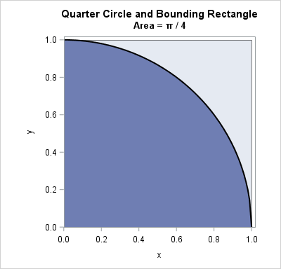
To compute Monte Carlo estimates of pi, you can use the function f(x) = sqrt(1 – x2). The graph of the function on the interval [0,1] is shown in the plot. The graph of the function forms a quarter circle of unit radius. The exact area under the curve is π / 4.
There are dozens of ways to use Monte Carlo simulation to estimate pi. Two common Monte Carlo techniques are described in an easy-to-read article by David Neal (The College Mathematics Journal, 1993).
The first is the "average value method," which uses random points in an interval to estimate the average value of a continuous function on the interval. The second is the "area method," which enables you to estimate areas by generating a uniform sample of points and counting how many fall into a planar region.
The average value method
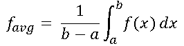
In calculus you learn that the average value of a continuous function f on the interval [a, b] is given by the following integral:
In particular, for f(x) = sqrt(1 – x2), the average value is π/4 because the integral is the area under the curve. In symbols,
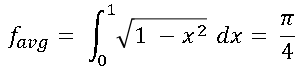
If you can estimate the left hand side of the equation, you can multiply the estimate by 4 to estimate pi.
Recall that if X is a uniformly distributed random variable on [0,1], then Y=f(X) is a random variable on [0,1] whose mean is favg. It is easy to estimate the mean of a random variable: you draw a random sample and compute the sample mean. The following SAS/IML program generates N=10,000 uniform variates in [0,1] and uses those values to estimate favg = E(f(X)). Multiplying that estimate by 4 gives an estimate for pi.
proc iml; call randseed(3141592); /* use digits of pi as a seed! */ N = 10000; u = randfun(N, "Uniform"); /* U ~ U(0, 1) */ Y = sqrt(1 - u##2); piEst1 = 4*mean(Y); /* average value of a function */ print piEst1; |

In spite of generating a random sample of size 10,000, the average value of this sample is only within 0.01 of the true value of pi. This doesn't seem to be a great estimate. Maybe this particular sample was "unlucky" due to random variation. You could generate a larger sample size (like a million values) to improve the estimate, but instead let's see how the area method performs.
The area method
Consider the same quarter circle as before. If you generate a 2-D point (an ordered pair) uniformly at random within the unit square, then the probability that the point is inside the quarter circle is equal to the ratio of the area of the quarter circle divided by the area of the unit square. That is, P(point inside circle) = Area(quarter circle) / Area(unit square) = π/4. It is easy to use a Monte Carlo simulation to estimate the probability P: generate N random points inside the unit square and count the proportion that fall in the quarter circle. The following statements continue the previous SAS/IML program:
u2 = randfun(N, "Uniform"); /* U2 ~ U(0, 1) */ isBelow = (u2 < Y); /* binary indicator variable */ piEst2 = 4*mean(isBelow); /* proportion of (u, u2) under curve */ print piEst2; |

The estimate is within 0.0008 of the true value, which is closer than the value from the average value method.
Can we conclude from one simulation that the second method is better at estimating pi? Absolutely not! Longtime readers might remember the article "How to lie with a simulation" in which I intentionally chose a random number seed that produced a simulation that gave an uncharacteristic result. The article concluded by stating that when someone shows you the results of a simulation, you should ask to see several runs or to "determine the variance of the estimator so that you can compute the Monte Carlo standard error."
The variance of the Monte Carlo estimators
I confess: I experimented with many random number seeds before I found one that generated a sample for which the average value method produced a worse estimate than the area method. The truth is, the average values of the function usually give better estimates. To demonstrate this fact, the following statements generate 1,000 estimates for each method. For each set of estimates, the mean (called the Monte Carlo estimate) and the standard deviation (called the Monte Carlo standard error) are computed and displayed:
/* Use many Monte Carlo simulations to estimate the variance of each method */
NumSamples = 1000;
pi = j(NumSamples, 2);
do i = 1 to NumSamples;
   call randgen(u, "Uniform");         /*  U ~ U(0, 1) */
   call randgen(u2, "Uniform");        /* U2 ~ U(0, 1) */
   Y = sqrt(1 - u##2);
   pi[i,1] = 4*mean(Y);        /* Method 1: Avg function value */
   pi[i,2] = 4*mean(u2 < Y);   /* Method 2: proportion under curve */
end;

MCEst = mean(pi);              /* mean of estimates = MC est */
StdDev = std(pi);              /* std dev of estimates = MC std error */
print (MCEst//StdDev)[label="Comparison of Methods"
                      colname={"Avg Func" "Area"}
rowname={"MC Estimate" "MC StdErr"}]; |
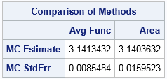
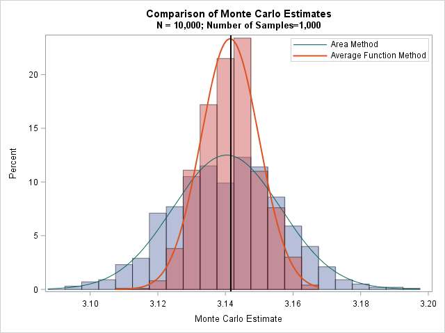
Now the truth is revealed! Both estimators provide a reasonable approximation of pi, but estimate from the average function method is better. More importantly, the standard error for the average function method is about half as large as for the area method.
You can visualize this result if you overlay the histograms of the 1,000 estimates for each method. The following graph shows the distribution of the two methods. The average function estimates are in red. The distribution is narrow and has a sharp peak at pi. In contrast, the area estimates are shown in blue. The distribution is wider and has a less pronounced peak at pi. The graph indicates that the average function method is more accurate because it has a smaller variance.
Estimating pi on Pi Day is fun, but this Pi Day experiment teaches an important lesson that is relevant 365 days of the year: If you have a choice between two ways to estimate some quantity, choose the method that has the smaller variance. For Monte Carlo estimation, a smaller variance means that you can use fewer Monte Carlo iterations to estimate the quantity. For the two Monte Carlo estimates of pi that are shown in this article, the method that computes the average function value is more accurate than the method that estimates area. Consequently, "on average" it will provide better estimates.

14 Comments
A Good Message:
Are the Monte Carlo Estimates UNBIASED Estimators ( of PI in this case )
That's a good question. The MC mean is a "mean of means," so theoretically it is an unbiased estimator. However, as I showed in this article, the results depend on the initial seed for the random number generator. Because we are using finite sample size and a finite number of samples, the initial seed could bias the result for a small-scale simulation. As the number of samples increases, this "seed bias" goes to zero.
Hi!
Great article! However I'm confused on a very fundamental point. I'll write it step by step for clarity.
We run the simulation for 1000 times each time we used 10.000 points. So we have an array of PI Estimates which has 1000 values in it.
Mean = avg(PI Estimates)
Standard Error of the Means = stdev(PI Estimates)*
or SEM = stdev(PI Estimates)/sqrt(1000**)*
* the problem of mine starts here. Which one is true and why?
** Notice that I typed 1000 which is the number of trials not 10.000.
Moreover how would you compute the error bars for 95% confidence interval. Is it +-1.96 * SE or SD?
I guess, the last question may become trivial depending on the answer of first one.
Thanks!
The first is correct.
MCMean = MC Estimate of mean = avg(PI Estimates) = average of the estimates over all simulations
MCSEM = MC Estimate of std error of mean = std(PI Estimates) = std dev of the estimates over all simulations
The formula that you write as SEM is (close to) the one-sample estimate of the SEM. If you take a single sample from the simulation and compute std(sample)/sqrt(10,000) then you should get a similar estimate for the precision of the mean. In particular, for the example in this article, you can compute
SEM1 = 4*std(Y) / sqrt(nrow(u));
or
SEM2 = 4*std(u2<Y) / sqrt(nrow(u));
for any of the 1000 samples. The 4 is because the function here is 4*mean.
To compute the CIs for a Monte Carlo estimate, use
MCMean +/- 1.96*MCSEM
Rick,
First of all thanks for your time and for the answer. I have to ask more to understand better. Here is what I did.
I made a small test to check the CI with MCSEM (as you said), I run the simulation for 1000 times then count means between CI for 95%. 948 of them lied in the interval. When I try for the second interval I gave above (as you interpret as wrong) 53 of the values lied in the interval.
So, roughly I can think this as we have a population (unknown), we take 1000 samples with sample size 10.000 for each. Right?
I run the simulation for one time (as you said) with 50.000 Dots. So, I have 1 sample with size 50.000. Let's call this case 1:
Mean 3.1287
Standard Error 0.0001
Median 3.1355
Mode 3.1111
Standard Deviation 0.0226
Then I run it 1000 times for 50.000 Dots. This is case 2:
Mean 3.1417
Standard Error 0.0002
Median 3.1418
Mode 3.1423
Standard Deviation 0.0071
Here is my question. If I understand correctly, SEM in case 1 (0.0001) is an estimate of the SD in case 2 (0.0071). This should lead me to CI(case 2) = (3.1278, 3.1556) (Mean +/- 1.96 * SD) which already covers 94.8% of the data.
And for case 1, by using SEM CI(case 1) = (3.1274, 3.1290) (Mean +/- 1.96 * SEM * 4(?**)) which only covers 0.19% of the data in case 2. What I am missing here? Obviously, 0.19% is not a good approximation, I am doing something wrong.
?** 4 didn't change much here, since SEM is 0.0001. Values I typed are without 4.
By the way, the distribution of case 1 (1 sample 50.000 dots) is not normal. (Kurtosis 267.456, Skewness 7.429) Is this related? Do I have to go for case 2 since its distributed pretty normal, thanks to Central Limit Theorem?
You seem to have many questions about simulation. The SAS Support Communities are a great place to ask questions, post your SAS code, and discuss statistical concepts. If you are using the DATA step, you can post to the Base SAS Support Community. (If you are using SAS/IML, post to the SAS/IML Support Community.)
Pingback: Monte Carlo estimates of joint probabilities - The DO Loop
Thanks for the suggestion but I don't use SAS. I found this blog through google. I'm going to answer my second question here, to help future visitors who might be confused. To make it short there was a bug in my code which is why I got 0.19% approximation instead of 95%.
Your first comment really helped me more than enough. Thanks again!
First off, interesting comparison between both methods and a very good point about variance, randomness, and reproducibility.
I have a question about the random interval [0,1], especially with regards to the area method. I take that notation to mean 0 and 1 are included in the interval and are valid outputs of randfun.
Wouldn't the points on the axis (only one of them, your choice) be counted double? If you look at the complete circle, then the correct range would be [-1,1], with the -1 and +1 included. If you divide it up into quarters, you would want to count only _one_ axis per quarter (say the +y for the quadrant shown in the post), because the other axis would be included in the other quadrants (say the +x axis with the next quadrant clockwise). And thinking like that would bring up the question whether to include the origin or not..
Anyway, my question is whether my interpretation of the effect of the random interval is correct? If so, how to handle it? Especially the origin? And would the average value method also be affected? (perhaps restrict the interval there to (0,1]? That is, 0 not included?)
Thanks for writing. You ask good questions.
1. In fact, the random number generator (RNG) I am using returns uniform variates in the open interval (0,1), so I should have written (0,1) instead of [0,1] in several places.
2. For area estimation, it doesn't matter whether you integrate the quarter circle function on the closed integral [0,1] or the open interval (0,1). The area under the unit circle is pi/4 whether you include the axes (and origin) or not. This is because the axes (and origin) are sets of "measure zero" in the 2-D plane.
3. From a Monte Carlo perspective, one or two extra points "inside" the circle are not going to change the estimate much compared to the standard error of the estimate. So it doesn't matter how you count a point that is on an axis. For that matter, you'll get a similar estimate whether you count a point as "in the circle" when x^2 + y^2 < 1 or whether you count "in" as x^2 + y^2 ≤ 1.
Thanks for answering, even though the thread is two-and-a-half years old!
Ad. 2: What does 'measure zero' mean? I'm decent at using math, but not that familiar with thinking about math. Maybe I'm thinking too analytically here, but is this basically the question on whether or not the borders of an area are included within that area or not? Same actually with the < resp. =< from your point 3.
Ad. 3: Given the nature of Monte Carlo and random numbers, I understand your point. Though, analytically again, in the limit for infinite points, I think there could still be a difference.
2. Measure theory is the mathematical foundation of probability. "Measure zero" means that lines and points have zero area. It doesn't matter whether you include lines and points when computing areas. For example, the area of the unit square and its boundary is 1. But also, the area of the unit square WITHOUT its boundary is 1! This shows that Area([0,1]x[0,1]) = Area([0,1]x[0,1]) = 1.
3. No, there is no difference. The probability of randomly selecting a point that is on the boundary is equal to the measure (area) of the boundary, which is zero.
Thanks for clearing that up. Like I said, I can use mathematics, but I don't know all the finer details and theories.
Someone asked how to illustrate this method by using the DATA step. The following DATA step simulates 1000 points in the square and colors them according to whether they are inside the unit circle: