I've written about how to generate a sample from a multivariate normal (MVN) distribution in SAS by using the RANDNORMAL function in SAS/IML software. Last week a SAS/IML programmer showed me a program that simulated MVN data and computed the resulting covariance matrix for each simulated sample. The purpose of the program was to study properties of the covariance matrices.
The programmer was pleased when I told him that SAS/IML software provides a simpler and more efficient way to simulate covariance and correlation matrices for MVN data. You can generate the covariance matrices directly by using the RANDWISHART function, which generates matrices from the Wishart distribution.
What is the Wishart distribution?
Before thinking about covariance matrices for multivariate normal data, let's recall a theoretical result for univariate data: For a sample of size n drawn from a normal distribution, the sample variance (appropriately scaled) follows a chi-square distribution with n–1 degrees of freedom. This means that if you want to study properties of the sample variance, you don't need to generate normal data. Instead you can draw a random chi-square variate and rescale it to produce a sample variance. No normal samples required!
This result generalizes to multivariate normal data. If you draw a sample from a MVN distribution with covariance matrix Σ, the sample covariance matrix (appropriately scaled) has a sampling distribution that is called the Wishart distribution. You can think of the Wishart distribution as a multivariate generalization of the chi-square distribution. It is a distribution of symmetric positive-definite matrices. A random draw from the Wishart distribution is some matrix that, upon rescaling, is a covariance matrix for MVN data.
From data to covariance matrices
Suppose that you want to approximate the sampling distribution of the correlation coefficient between two correlated normal variables in a sample of size 50. The straightforward approach is to simulate 50 observations from the bivariate normal distribution, compute the correlation coefficient for the sample, and then repeat the process many times in order to approximate the distribution of the correlation coefficients. An implementation in PROC IML follows:
proc iml;
call randseed(12345);
N = 50;                              /* MVN sample size   */
Sigma = {9 1,                        /* population covariance; correlation = 1/3 */
         1 1};
NumSamples = 1000;                   /* number of samples in simulation */

/* First attempt: Generate MVN data; compute correlation from data */
corr = j(NumSamples, 1, .);          /* allocate space for results */
do i = 1 to NumSamples;
   X = randnormal(N, {0 0}, Sigma);  /* MVN sample of size 50 */
   corr[i] = corr(X)[2];             /* corr = off-diagonal element */
end;

title "Distribution of Correlation Coefficient";
title2 "N=50; rho = 1/3";
call histogram(corr) xvalues=do(-2,0.7,0.1)
other="refline 0.333 / axis=x"; |
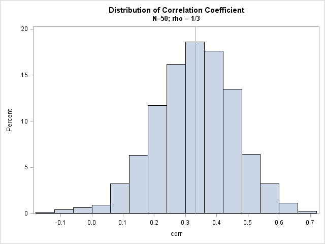
The histogram shows the approximate sampling distribution for the correlation coefficient when the population parameter is ρ = 1/3. You can see that almost all the sample correlations are positive, a few are negative, and that most correlations are close to the population parameter of 1/3.
Sampling from the Wishart distribution in SAS
In the previous section, notice that the MVN data is not used except to compute the sample correlation matrix. If we don't need it, why bother to simulate it? The following program shows how you can directly generate the covariance matrices from the Wishart distribution: draw a matrix from the Wishart distribution with n–1 degrees of freedom, then rescale by dividing the matrix by n–1.
/* More efficient: Don't generate MVN data, generate covariance matrix DIRECTLY! Each row of A is scatter matrix; each row of B is a covariance matrix */ A = RandWishart(NumSamples, N-1, Sigma); /* N-1 degrees of freedom */ B = A / (N-1); /* rescale to form covariance matrix */ do i = 1 to NumSamples; cov = shape(B[i,], 2, 2); /* convert each row to square matrix */ corr[i] = cov2corr(cov)[2]; /* convert covariance to correlation */ end; call histogram(corr) xvalues=do(-2,0.7,0.1); |
The histogram of the correlation coefficients is similar to the previous histogram and is not shown. Notice that the second method does not simulate any data! This can be quite a time-saver if you are studying the properties of covariance matrices for large samples with dozens of variables.
The RANDWISHART distribution actually returns a sample scatter matrix, which is equivalent to the crossproduct matrix X`X, where X is an N x p matrix of centered MVN data. You can divide by N–1 to obtain a covariance matrix.
The return value from the RANDWISHART function is a big matrix, each row of which contains a single draw from the Wishart distribution. The elements of the matrix are "flattened" so that they fit in a row in row-major order. For p-dimensional MVN data, the number of columns will be p2, which is the number of elements in the p x p covariance matrix. The following table shows the first five rows of the matrix B:
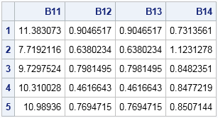
The first row contains elements for a symmetric 2 x 2 covariance matrix. The (1,1) element is 11.38, the (1,2) and (2,1) elements are 0.9, and the (2,2) element is 0.73. These sample variances and covariances are close to the population values of 9 1, and 1. You can use the SHAPE function to change the row into a 2 x 2 matrix. If necessary, you can use the COV2CORR function to convert the covariance matrix into a correlation matrix.
Next time you are conducting a simulation study that involves MVN data, think about whether you really need the data or whether you are just using the data to form a covariance or correlation matrix. If you don't need the data, use the RANDWISHART function to generate matrices from the Wishart distribution. You can speed up your simulation and avoid generating MVN data that are not needed.

3 Comments
Dear Rick Wicklin,
you said "The RANDWISHART distribution actually returns a sample scatter matrix, which is equivalent to the crossproduct matrix X`X, where X is an N x p matrix of centered MVN data."
I want to know about X (variable(x1, x2) in Wishart distribution) use for Goodness-of-fit tests for multivariate normality?
You'll have to be more specific. There are dozens of tests for multivariate normality. The crossproduct matrix alone is not sufficient for determining multivariate normality, since many distrivutions could have the same crossproduct matrix. However, the crossproduct matrix is used to form the covariance matrix, which is used to form Mahalanobis distances from observations to the multivariate mean. In MVN data, the distances fallow a chi-square distribution, and that can be used as a test of MVN normality.
Dear Rick Wicklin,
If X is a multivariate distribution, the sample size is 10, the number of variables is 3, the simulating data from multivariate gamma distribution (Wishart distribution). The result is 9 columns and 10 observations. Which x1, x2 and x3 are used for testing multivariate normal distribution by jaque-bera test.
What is x1,x2,x3 in 9 columns?
Thank you in advance and Best Regards,
Mantana Seeno