This week I read an interesting blog post that led to a discussion about specifying the frequencies of observations in a regression model. In SAS software, many of the analysis procedures contain a FREQ statement for specifying frequencies and a WEIGHT statement for specifying weights in a weighted regression. Theis article takes a quick look at the FREQ and WEIGHT statements in regression models, and when you should use one instead of the other.
The difference between frequencies and weights in regression analysis Click To TweetSpecifying frequencies
Frequencies are not weights, although they are similar enough that confusion is inevitable. SAS customers ask about the difference so often that SAS Technical Support has a usage note on the distinction between the WEIGHT and FREQ statements in SAS. It is important for statistical software to support both methods.
In short, a "frequency variable" is one that specifies an integer count that is associated with each observation. The SAS documentation is filled with examples of specifying a frequency variable. For example, see the examples for the LOGISTIC procedure.
Here are some key points to remember:
- A frequency variable tells the procedure that there are more observations than there are rows in the data set.
- When you run a frequency analysis, your analysis should agree with the same analysis run on the "expanded data," which is the data set in which each row represents a single observation.
- A frequency variable changes the degrees of freedom in the model. This affects many statistics: means, standard errors, p-values, and so forth.
As an example, I will use the data from the Freakonometrics blog:
data FreqData; input x y Count @@; datalines; 18 14 74 18 19 13 18 21 7 18 23 1 23 14 6 23 19 4 23 21 2 23 23 7 23 25 4 25 14 2 25 19 3 25 21 2 25 23 2 25 25 4 27 14 1 27 19 1 27 21 2 27 23 3 27 25 3 27 27 2 29 14 2 29 21 1 29 23 3 29 25 2 29 29 6 31 14 2 31 21 2 31 23 1 31 29 1 31 31 2 31 33 1 33 23 2 33 29 1 33 31 1 33 33 3 35 19 1 35 23 1 35 33 2 37 25 1 37 27 1 37 31 1 37 35 1 ; |
The data contains an explanatory variable (X), a response variable (Y), and a frequency variable (Count). Assume that the goal is to perform a linear regression for these data.
First, let's expand the data by using the frequency variable. The FreqData data set has 42 observations, but the following SAS DATA step creates a data set named Expand that has 181 observations, which is the sum of the Count variable:
/* Expand original data by frequency variable */
data Expand;
keep x y;
set FreqData;
if Count<1 then delete;
do i = 1 to int(Count);
   output;
end;
run;

proc sgplot data=Expand;
scatter x=x y=y / markerattrs=(symbol=CircleFilled size=12)
                  transparency=0.7;  /* in SAS 9.4, use the JITTER option! */
run; |
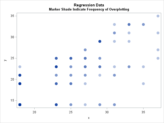
In the scatter plot, many markers are overplotted. For example, the marker at (18, 14) is plotted 74 times. Transparency is used to show that some values are repeated multiple times in the data. In addition, you might want to use jittering to help visualize overplotting in scatter plots. In SAS 9.4, there is a new JITTER option on the SCATTER statement, which makes jittering much easier than in SAS 9.3.
Now that the data are expanded, let's compute a simple linear regression of Y on X and look at some of the output. This is the "gold standard" to which we will compare other attempts.
ods graphics off; ods select NObs(persist) ANOVA(persist) ParameterEstimates(persist); proc reg data=Expand; model y=x; run; |
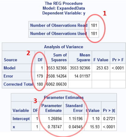
You can click on the image to enlarge it. Three parts of the results are circled in red:
- The number of observations used in the analysis: n = 181
- The degrees of freedom: We are estimating two parameters, so there are n − 2 = 179 degrees of freedom for the error term
- The parameter estimates are b0 = 1.269 and b1 = 0.787, and the standard errors (which depend on the degrees of freedom!) are as shown.
As I stated previously, we should get these same results when we use the FREQ statement on the original data, as follows:
proc reg data=FreqData; freq Count; model y=x; run; |
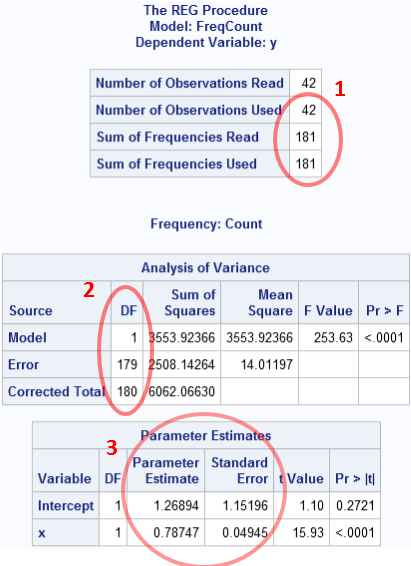
Success! The statistics for this computation are identical to the statistics for the expanded data. The only difference is that the data set has 42 observations, but the FREQ statement results in a "Sum of Frequencies" equal to 181. That number is used as the sample size (n) in the degrees of freedom computations.
Specifying weights
Weights are not frequencies. The WEIGHT statement does not change the "sample size" or the "degrees of freedom."
You can use a WEIGHT statement when you some observations contribute to the model fit more than others. A canonical example of this is that if you identify outliers in your data, you can assign them weights that are zero or nearly zero in order to obtain a fit that is robust to the outliers. As this example indicates, weights do not have to be integers. You can also use weights when some response values are known more precisely than others. In that case, it is common to weight each observation proportional to the inverse of the variance of that observation. These are known as inverse-variance weights or accuracy weights.
In the regression context, if you use integer counts as weights, the parameter estimates are the same as when you use the counts for frequencies, but the statistics that use the sample size are different. This includes standard errors for the estimates and p-values for significance. This is shown in the following example:
proc reg data=FreqData; weight Count; model y=x; run; ods select all; |
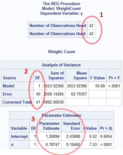
As you can see, the analysis thinks that there are only 42 observations. Although the parameter estimates are correct, almost all of the other statistics are wrong (assuming that you are trying to reproduce the analysis for the expanded data).
So the conclusion is that you should use the FREQ statement to specify integer frequencies for repeated observations. Use the WEIGHT statement when you want to decrease the influence that certain observations have on the parameter estimates.

9 Comments
Thanks for the very instructive posting. Is there any reason why observation counts specified with the FREQ variable need to be integers? And is there any way to bypass this restriction?
For example, suppose I observe colors and I know that there is 60% chance that the observed color was red, and a 40% chance that it was green. I might then want to encode this uncertainty by encoding the single observation as two rows: a "red" row with FREQ-value 0.6 and a "green" row with FREQ-value 0.4. I cannot do that with the FREQ statement because of the integer restriction. But can I do it with the WEIGHT statement instead, if I am only interested in the parameter estimates, even though I cannot trust the other reported statistics then? And will it work for all distributions and procedures that use maximum-likelihood optimation (eg, GENMOD / GLIMMIX), or only some of them? or is there a better way of achieving the same result?
The FREQ variable should be an integer because it is shorthand for specifying the number of rows that this observation represents. That is the definition (or interpretation, if you prefer) of a frequency variable.
Data sets contain observed values, not probabilities. You observe, count a certain number of each color, and then analyze the results. You can ask questions like "are my data consistent with the hypothesis that red occurs 60% of the time." Many statistics depend on the sample size to determine inference and uncertainty. In your example, how many colors are observed? The number of observations is the sum of the FREQ variable, so your example is telling me that you observed 0.6 + 0.4 = 1 value. Unfortunately, you can't do statistics on one observation. And what was the color that you observed? Your example does not specify it.
Yes, you can use the WEIGHT variable to encode uncertainty, and the article describes how to interpret weights. In particular, your example would have two observations, but the "red" row would have greater influence on the parameter estimates than the "green" row. But I suspect that this is not what you are trying to acheive.
For instance, there are two sentences:
a) 'Sam!’
b) 'A loud ringing of one of the bells was followed by the appearance of a smart chambermaid in the upper sleeping gallery, who, after tapping at one of the doors, and receiving a request from within, called over the balustrades -'Sam!'.'
Evidently, that the 'Sam' has different importance into both sentences, in regard to extra information in both. This distinction is reflected as the phrases, which contain 'Sam', weights: the first has 1, the second – 0.08; the greater weight signifies stronger emotional ‘acuteness’; where the weight refers to the frequency that a phrase occurs in relation to other phrases.
Pingback: Weighted percentiles - The DO Loop
Pingback: Visualize a weighted regression - The DO Loop
Pingback: How to understand weight variables in statistical analyses - The DO Loop
Thank you. I am trying to understand the weight statement in logistic regression versus proc reg.
For logistic regression, it seems "weight" works the same as "freq" for integer counts. Multiplying weight or freq will drive the result to significance. However, for proc reg, the two give different results, multiplying weight still gives the same result.
Could you give some explanation about the difference in logistic regression?
The documentation gives the formulas for the parameter estimates. For many statistics, the formulas for are symmetric in the frequencies and weights. However, the sample size is the sum of the frequencies, so any statistics that use the sample size or degrees of freedom will be different. For example, the Schwarz criterion (SC) and the Average Squared Error uses the sample size. Use the GOF option on the MODEL statement and inspect the Model Fit Statistics table for each model.
Pingback: The difference between frequencies and weights in a correlation analysis - The DO Loop