I've been a fan of statistical simulation and other kinds of computer experimentation for many years. For me, simulation is a good way to understand how the world of statistics works, and to formulate and test conjectures. Last week, while investigating the efficiency of the power method for finding dominant eigenvalues, I generated symmetric matrices to use as test cases. Each element of the matrix was drawn randomly from U[0,1], the uniform distribution on the unit interval. As I checked my work for correctness, I noticed a few curious characteristics about the eigenvalues of these matrices:
- They have one positive dominant eigenvalue whose value is approximately n/2, where n is the size of the matrix.
- The other eigenvalues are distributed in a neighborhood of zero.
I noticed that the same pattern held for all of my examples, so I turned to simulation to try to understand what was going on.
The distribution of eigenvalues in random matrices
I had previously explored the distribution of eigenvalues for random orthogonal matrices and shown that they have complex eigenvalues that are (asymptotically) distributed uniformly on the unit circle in the complex plane. I suspected that a similar mathematical truth was behind the pattern I was seeing for random symmetric matrices.
The key statistical observation is that if the elements of a matrix are random variables, then the eigenvalues (which are the roots of a polynomial of those elements) are also random variables. As such, they have an expected value and a distribution. My conjecture was that the expected value of the largest eigenvalue was n/2 and that the expected values of the smaller eigenvalues are clustered near zero.
In a series of simulations, I generated a large number of random symmetric nxn matrices with entries drawn from U[0,1]. For each matrix I computed the n eigenvalues and stored them in a matrix with n columns. Each row of this matrix contains the eigenvalues for one random symmetric matrix. The ith column contains simulated values for the position of the ith eigenvalue. (Recall that the EIGEN routine in SAS/IML software returns the eigenvalues in (descending) sorted order.) The following graph shows the distribution of eigenvalues for 5,000 random symmetric 10x10 matrices:
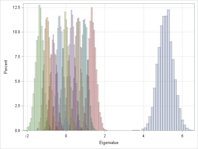
Each color represents an eigenvalue, and the histogram of that color shows the distribution of the eigenvalue for 5,000 random 10x10 matrices. Notice that the largest eigenvalue is always close to 5. The largest eigenvalue has a distribution that looks like it might be approximately normally distributed. The distributions for the smaller eigenvalues overlap. A typical 10x10 matrix has 4 smaller positive eigenvalues, 4 smaller negative eigenvalues, and one eigenvalue whose expected value seems to be close to zero.
You can convince yourself that this result is reasonable by considering the constant matrix, C, for which every element is identically 0.5. (I got this idea from a paper that I will discuss later in this article.) This matrix C is singular with n-1 zero eigenvalues. Because the sum of the eigenvalues is the trace of the matrix, C has a single positive eigenvalue with value n/2. The random matrices that we are considering have an expected value of 0.5 in each element, so it makes sense that the eigenvalues will be close to the eigenvalues of C.
What happens for large matrices?
I did a few more simulations with matrices of different sizes. The patterns were similar. I suspected that there was an underlying mathematical theorem at work. As for orthogonal matrices, I conjectured that the theorem was probably an asymptotic result: as the size of the matrix gets large, the eigenvalues have certain statistical properties. To test my conjecture, I repeated the simulation for random 100x100 matrices. The following graph shows the distribution of the eigenvalues for 5,000 simulated matrices:
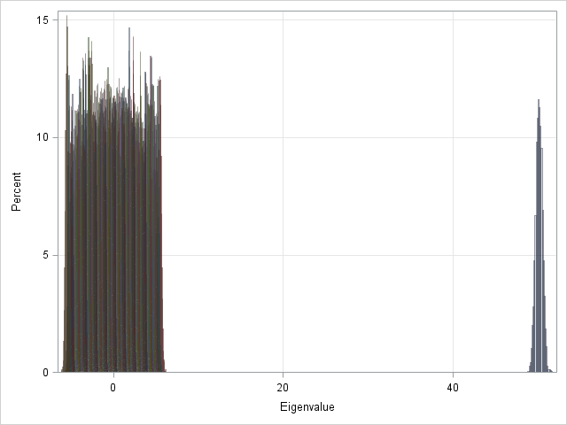
The scale of the plot is determined by the distribution of the eigenvalue near 50=100/2. The other histograms are so scrunched up near zero that you can barely see their colors.
To better understand the expected values of the eigenvalues, I computed the means of each distribution. These sample means estimate the expected values of the eigenvalues for n=100. For my simulated data, I found that the dominant eigenvalue is centered at 50.16. The confidence interval for that estimate does NOT include 50, so I would conjecture that the eigenvalue approaches n/2 from above.
If you plot a histogram of the non-dominant eigenvalues, you get the following graph:
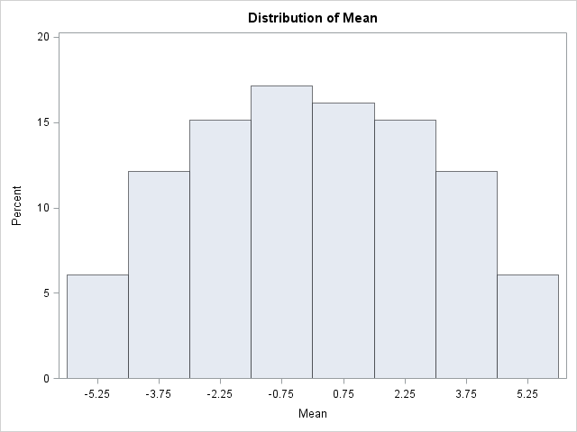
When I saw the shape of that histogram, I was surprised. I expected to see a uniform distribution. However, my intuition was mistaken and instead I saw a shape that curves down sharply at both ends. After I generated eigenvalues for even LARGER matrices, I commented to a colleague that "it looks like the density is semi-circular." However, I had never encountered a semi-circular distribution before.
Conjecture confirmed!
At the end of my previous article, I mentioned a few of these conjectures and asked if anyone knew of a theorem that describes the statistical properties of the eigenvalues of a random symmetric matrix. Remarkably, I had an answer within 24 hours. Professor Steve Strogatz from Cornell University, commented as follows:
Each entry for such a matrix has an expected value of mu= 1/2, and there's a theorem by Furedi and Komlos that implies the largest eigenvalue in this case will be asymptotic to n*mu. That's why you are getting n/2. And the distribution of eigenvalues (except for this largest eigenvalue) will follow the Wigner semicircle law.
The reference Strogatz cites is a 1981 article in Combinatorica titled "The eigenvalues of random symmetric matrices." The first sentence of the paper is "E. P. Wigner published in 1955 his famous semi-circle law for the distribution of eigenvalues of random symmetric matrices." I suppose "famous" is a relative term: I had never heard of the "Wigner semicircle distribution," but it is famous enough to have its own article in Wikipedia.
The paper goes on to formulate and prove theorems concerning the eigenvalues of random symmetric matrices. The theorems explain the phenomena that I noticed in my simulations, including that the dominant eigenvalue is approximately normally distributed and its expected value converges to n/2 from above. See the paper for further details.
SAS Programs for simulation and analysis
If you would like to conduct your own simulations, this section includes the SAS/IML program used to generate the symmetric random matrices. Although I generated the elements from U[0,1], Wigner's result holds for any distribution of elements, as do the results of Furedi and Komlos. The following program writes the eigenvalues to a SAS data set with 5,000 rows and n variables named e1, e2, ..., en. The value of n is determined by the size macro variable.
%let size=10;  /* controls the size of the random matrix */
proc iml;
/* find eigenvalues of symmetric matrices with A[i,j]~U(0,1) */
NumSim = 5000;
call randseed(1);

n = &size;
r = j(n*(n+1)/2, 1);/* allocate array for symmetric elements */
results = j(NumSim, n);
do i = 1 to NumSim;
   call randgen(r, "uniform"); /* fill r with U(0,1) */
   A = sqrvech(r);             /* A is symmetric */
   eval = eigval(A);           /* find eigenvalues */
   results[i,] = eval`;        /* save as ith row */
end;

labl = "e1":("e"+strip(char(n))); /* var names "e1", "e2", ... */
create Eigen from results[c=labl];
append from results;
close Eigen;
quit; |
The following SAS program is used to analyze the eigenvalues, including making the graphs shown in this article.
/* make a histogram statement for e1-e&n */ %macro eigenhist(n); %do i = 1 %to &n; histogram e&i / transparency = 0.7; %end; %mend; /* overlay distributions of e1-e&size */ proc sgplot data=eigen noautolegend; %eigenhist(&size); yaxis grid; xaxis grid label="Eigenvalue"; run; /* dist of expected values */ /* compute mean of each variable (or use PROC SQL or PROC MEANS...) */ proc iml; use eigen; read all var ("e1":"e&size") into X; close eigen; mean = T(mean(X)); rank = T(do(&size,1,-1)); /* 100, 99, ..., 1 */ create EigMeans var {"rank" "Mean"}; append; close EigMeans; quit; proc univariate data=EigMeans; where rank<&size; var Mean; histogram Mean; run; |

3 Comments
Hi Rick
I hope this note finds you well this morning. I think you will be even more intrigued by random matrices (especially Hermitians) and associated eigenvalues after reading this piece on tantalizing links between matrix eigenvalues distributions, nuclear physics and Riemann's zeta zeros http://web.williams.edu/go/math/sjmiller/public_html/RH/Hayes_spectrum_riemannium.pdf
Have a great day
Daniel
Daniel
Terrence Tao has a number of recent articles about Wigner matrices. Many (all?) of them are available online at http://terrytao.wordpress.com/
I make no claim of understanding this stuff myself! ;-)
Pingback: Creating an array of matrices - The DO Loop