This blog post shows how to numerically integrate a one-dimensional function by using the QUAD subroutine in SAS/IML software. The name "quad" is short for quadrature, which means numerical integration.
You can use the QUAD subroutine to numerically find the definite integral of a function on a finite, semi-infinite, or infinte domain. In order to use the QUAD subroutine, you must be able to write down an expression for the function that you want to integrate. The QUAD subroutine evaluates the expression at certain locations (chosen by the algorithm) so that the integral is computed to a high level of accuracy with relatively few function evaluations.
In order to use the QUAD subroutine, you must supply at least two input arguments and one output argument. The simplest syntax for the QUAD subroutine is
call quad(result, "FcnName", limits);where the arguments are as follows:
- result is an output argument that will contain the value of the integral
- "FcnName" is the name of a SAS/IML function module that evaluates the integrand at an arbitrary point within the limits of integration
- limits defines the limits of integration
A Simple Integral
For a simple example, suppose that you want to integrate the cosine function over the interval [a, b]. The following SAS/IML module, MyFunc, evaluates the integrand at an arbitrary point:
proc iml; start MyFunc(x); return( cos(x) ); finish; |
In order to integrate the cosine function over, say, the interval [0, π/2], use the following statements:
/** integrate cos(x) on [a,b] **/
a = 0;
b = constant("PI") / 2;
call quad(R, "MyFunc", a||b); |
The value of the integral is stored in the 1x1 scalar R. For this example, you can compare the numerical result to the exact value of the integral by using the indefinite integral (which is the sine function):
/** compare with exact answer */ exactInt = sin(b) - sin(a); diff = exactInt - R; print R exactInt diff; |
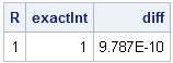
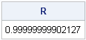
The numerical result is within 10-9 of the exact value. By default, SAS/IML prints values by using a BEST9. format, so the value of R is displayed as 1. To see more digits of precision, you can explicitly specify a w.d format in the PRINT statement:
print R[format=16.14]; |
How Does the QUAD Subroutine Work?
In a broad sense, there are two type of numerical integration routines: those that integrate data and those that integrate functions. The trapezoidal rule and Simpson's rule are examples of techniques that can approximate the integral when given data in the form of (x, y) pairs. These techniques are not adaptive; they use the data points that they are given. I will discuss these methods in a future blog post.
In contrast, the numerical method used by the QUAD subroutine requires a function that can be evaluated at any point in the domain of integration.
The QUAD routine implements a Romberg-type integration scheme. In its simplest form, Romberg integration is a numerical integration method that uses extrapolation of trapezoidal sums to approximate an integral over a domain. Roughly speaking, Romberg's method computes a sequence of trapezoidal approximations with decreasing step sizes, and extrapolates the result to the limiting case of zero step size. The QUAD subroutine is actually more sophisticated than this and implements additional features for dealing with singularities, functions with large derivatives, and infinite domains.
The SAS/IML documentation has further details on the QUAD subroutine and includes examples of integration over infinite and semi-infinite domains. You can also use the QUAD routine to evaluate a double (iterated) integral.

18 Comments
Pingback: Obtaining area from a set of points on a curve - The DO Loop
can we perform multiple integration (with a higher dimension than double) using SAS?
The standard technique for high-dimensional integration is to use Monte Carlo methods. If you are asking this question in a Bayesian context, look at the MCMC procedure in SAS.
what if I want to make a double integration for which I don’t have an expression for the function I want to integrate. In other words, suppose my integrand is “C” where “C” is computed through many steps including probabilities, transpose, and inverse of matrices until we reach a value of “C”. Also, C takes different values according to the values in the domain of the integration variable. How could I do this in SAS?
It sounds like you would want to use Monte Carlo or quasi-Monte Carlo intergation in two dimensions. For background information, see the lecture notes at http://sas.uwaterloo.ca/~dlmcleis/s906/, especially Chapter 6: Quasi-Monte Carlo Multiple Integration
Does this mean that I could do the integration I need in SAS?
It means that it can be done in SAS, yes. However, I don't have any pre-written code that I can send you. I don't know your statistical and programming background, so I don't know whether you would find it easy or difficult.
Refering to my previous question, could i write the double integration as a double summation using guass hermite and laguerre functions(as i have y ^alpha *e(-y) and e(-x*x) in the integrand ), calculate the quadrature points and weights and then double loop over the quadrature points of x and y and after the double loop ends i will get the double integtation value?
Refering to my previous question, could i write the double integration as a double summation using guass hermite and laguerre functions(as i have y ^alpha *e(-y) and e(-x*x) in the integrand ), calculate the quadrature points and weights and then double loop over the quadrature points of x and y and after the double loop ends i will get the double integtation value?
Sample program # 40592 shows how to use QUAD in DATA or PROC steps via PROC FCMP.
I would like to use it in defining an objective function for an optimization. I am concerned that requiring each evaluation of my objective function to re-initiate PROC IML will cause scalablity problems for my optimization.
Are there any plans to make something like QUAD available directly to the rest of SAS without constant re-initiation of IML?
Short answer, "no." Longer answer: I recommend that you do the optimization in IML, along with the integration. My blog has several optimization examples.
Dear Dr. Wicklin,
I want to write SAS code for numerical integration of a function of two variables to run the bigger SAS program in the aim of performing iterative procedure of estimation of optimal bandwidth in non-parametric regression analysis. How I can send you the function to you, which is to be typed in equation editor.
Regards,
Himadri Ghosh,
Principal Scientist,
Indian Agricultural Statistics Research Institute,
PUSA, New Delhi-110012
INDIA
You can post questions like this to the SAS/IML Support Community. The forum supports uploading files, including images, PDFs, etc. You might also want to read this article about how to optimize a function of an integral.
Pingback: Reversing the limits of integration in SAS - The DO Loop
Pingback: The value of pi depends on how you measure distance - The DO Loop
Pingback: Estimate an integral by using Monte Carlo simulation - The DO Loop
Pingback: Avoid domain errors by using Taylor series - The DO Loop
Pingback: An exact formula for the sampling distribution of the correlation coefficient - The DO Loop