Following on from my last blog introducing the series, in this section, we’ll take a first look at Explanatory Data Analysis with basic summary statistics.
Getting started with a new dataset in analytics can be daunting. It can help when first looking at a dataset to start with basic summary statistics. This shows us the distribution of values as well as the moments around the mean. This can be important for a few reasons. Firstly, we can evaluate the ranges of numeric values and how much they vary from their series mean. This is an important point when using Predictive Analytics as, typically, you want numeric attributes to be on a similar scale as the other inputs. For models which rely on numeric attributes using a similar scale, such as Neural Networks, it may be worth using a standardization or normalization technique to re-scale inputs.
For example, looking at the summary statistics in Table 1 for the numeric attributes in HMEQ, we can see that the value ranges are difficult to compare. An outstanding mortgage amount is naturally going to be on a different scale to years of job experience (YOJ).

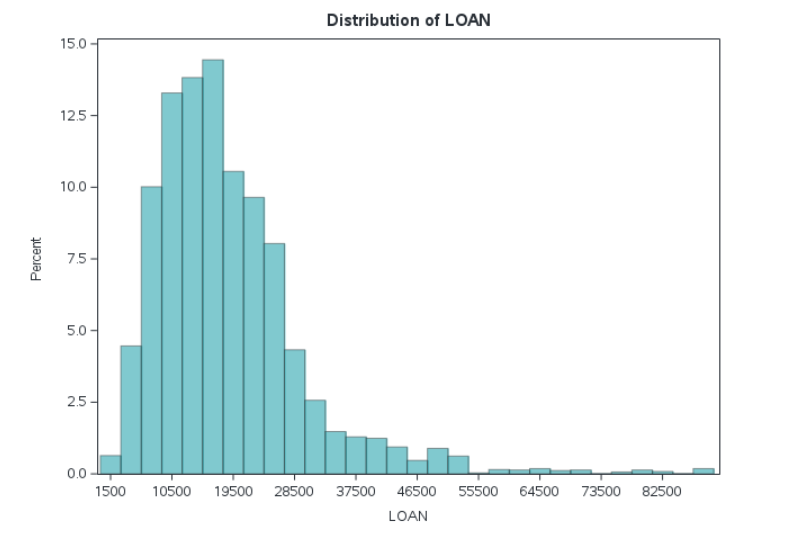
Likewise, numeric attributes which have a skewed or non-normal distribution may benefit from a transformation, such as converting to a logarithmic scale. For example, looking at Figure 1, with the loan we see there is a range of roughly $1,000 to $90,000. Most values fall between $10,000 and $20,000. There appears to be a long tail on the right of the distribution (i.e. skewed distribution), with few outlier loan amounts for very large sums.
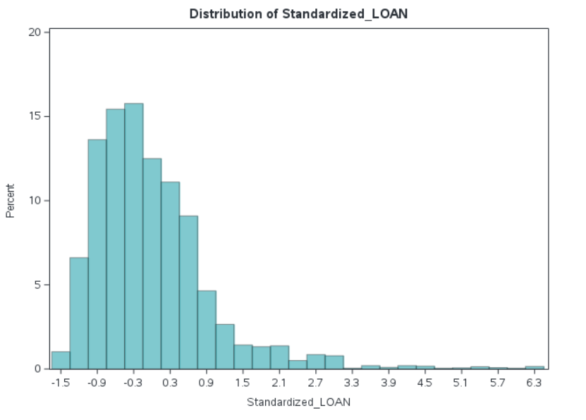
If we standardize our data using the standard deviation (subtract the mean and divide by the standard deviation) then we can retain the same shape of the data on a normalized scale, which we can see in Figure 2. This makes it easier to include multiple variables into a model which have very different scales. Note this does not remediate any skewness in our data.
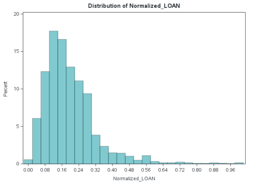
Another form of feature scaling technique we can employ is to scale the data into a range between 0 and 1. This is known as Normalization and is shown in Figure 3. As with Standard Deviation based standardization, we retain the original shape of the data, warts and all.
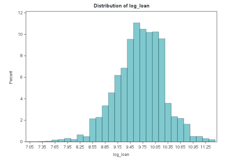
We can see in Figure 4 that when we transform this variable via logarithmic scaling the skewness of the distribution is no longer an issue and it appears approximately normally distributed, which may be helpful in some modeling scenarios as well as allowing us to perform other statistical analyses with the data.
You may need to consider other transformation methods depending on your dataset. For example, if we needed to transform YOJ it is plausible that someone has zero years in the role – in this case, we cannot use a log transformation (since log(0) = -Infinity) so we would need to consider something different like using a Square Root transformation on the series. With our example variable, LOAN, it is highly unlikely that anyone would apply for a loan amount of $0 so we can use a log transformation. We need to be careful here though as it is generally a bad statistical practice to ‘cherry pick’ methods or techniques.
Looking back at the summary statistics we can see that 60% of our numeric variables have a minimum value of zero, so for this particular data set log transformations are, in fact, not particularly useful.
Generally, the default choice of transformation is to log scale data. If we wanted to use log transformation and if, for example, YOJ was the only variable that contained zeros, we might consider converting it to a categorical variable based on bins of experience (0-5 years, 5-10 years, etc.).
This leads to a broader consideration around Feature Engineering, where we consider methods to transform our variables in a way that might yield more accurate predictive models, such as binning numeric attributes so that they are treated as categorical inputs. We’ll cover more on this in the next blog when we discuss Predictive Modelling.
Assessing the target distribution
Generally speaking, most Supervised Machine Learning models expect to learn the patterns of either numeric or categorical targets, these are referred to respectively as regression and classification.
Many of these models are parametric – i.e. they assume a distribution for the target variable. If we take for example a Simple Linear Regression model, there is an assumption that the dependent variable we are trying to predict is normally distributed around its relationship with the independent variable. As with the numeric inputs to the model, when working with predictive analytics it may be prudent to transform the target variable for training your model, for example, log transformations make multiplicative relationships additive, which can be easier to work with.
When considering a classification model, there are other considerations to keep in mind. For example, with our HMEQ dataset, we are building a model to predict whether someone will default on a loan. We can firstly think about the event levels of our target where 1 means they did default on their loan. If we want to predict that they will default, then 1 is our positive class. This may not sound like an important distinction, but if we treat 0 as the positive class then our model may not be as accurate as it will be optimizing predicting whether someone will not default on a loan.
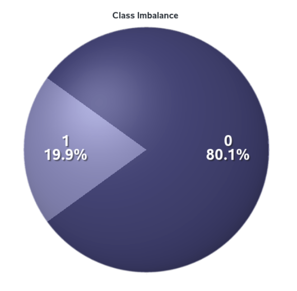
In the context of fraud and error modeling it is important to note that often the positive class will be a rare event. This is intuitive since if it was not rare for people to default on their loans then there may not be many banks still in business! As part of the exploratory analysis, it is therefore important for us to assess the proportions of our target class levels and assess whether we need to use some event-based stratified sampling, or even oversampling of the positive class. Figure 5 shows that for our HMEQ dataset, the target variable has an imbalanced class – suggesting we would need to consider event-based sampling methods when we begin building predictive models.
In the next blog, we'll discuss correlation.
Check out the work of fellow data scientists on Data Science Experience hub. www.sas.com/datascienceexperience