Changing how we’ve viewed the beautiful game forever.
How often have we looked at a game and wondered, “How did he miss that?!” Now, with expected goals (xG) metric, we can really see if our frustration is justified, and perhaps use that to predict future results.
The use of analytics in sport is not a new concept. The average NBA fan is more likely than ever to use statistics to understand a game. The mainstream media uses widely available statistics for discussion, including points, assists, blocks, steals, percentage field goals, free throw differentials and much more. Whereas your average football fan would say “my eyes tell me everything I need to know” due to the longtime misuse of statistics by fans.
What is expected goals?
Opta, the leading football data provider, describes xG as “the quality of a shot based on several variables such as assist type, shot angle and distance from goal, whether it was a headed shot and whether it was defined as a big chance.” In other words, it uses historical averages to determine how likely it is that a chance should be scored. Adding together all these numbers can indicate how many chances should have been scored, on average.
Why?
The xG metric allows us to look at the underlying performance compared to actual results with the naked eye. It helps us comprehend the game, and if used correctly, to predict future outcomes more accurately than any other measure.
Mo Salah's 'decline'
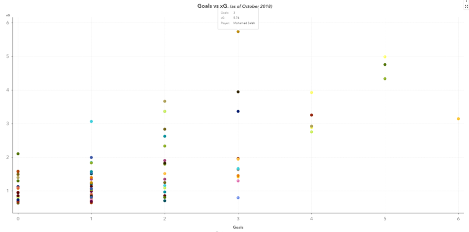
When Mo Salah scored a record-breaking 32 goals to become Premier League top scorer of the 2017/18 season, expectations were high for him to hit the ground running. However, when he only scored three goals in eight games by mid-October, many described him as a “one-season wonder” and unable to replicate last season’s form.
Using SAS Visual Analytics, we were able to look at the xG metric. Mo Salah was, in fact, leading the league with expected goals (displayed on the y-axis), yet he wasn’t anywhere near the top scorers (x-axis), where eight players had scored more than him. This suggested he was merely underperforming (or unlucky) rather than in decline.
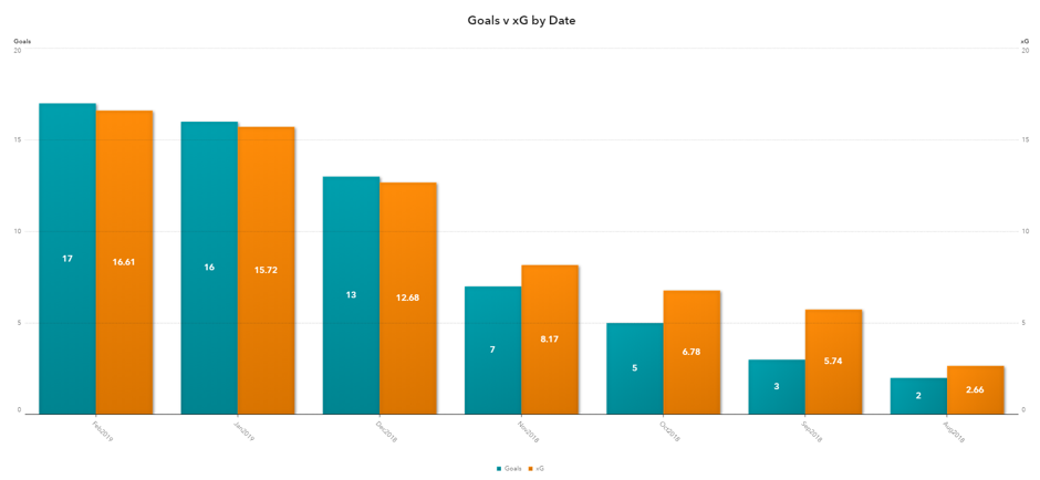
Forward four months and 17 league games. Mo Salah now sits joint at the top of the Premier League scorers chart. You can see from the chart below how he’s managed to align to his expected goals. Underlying performances could suggest more than just the output, over the long run.
Future expectations
Just as we get 50:50 results between heads/tails when tossing a coin over a large sample size, xG tends to level out with actual goals scored.
Another example of how expected goals can ‘predict the future’ is the case of the iconic Leicester striker Jamie Vardy, who finished the 2017/2018 Premier League season with an impressive 20 goals. But what did his numbers suggest?
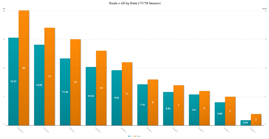
We can see from the above chart that Jamie Vardy outperformed his xG by nearly five goals!
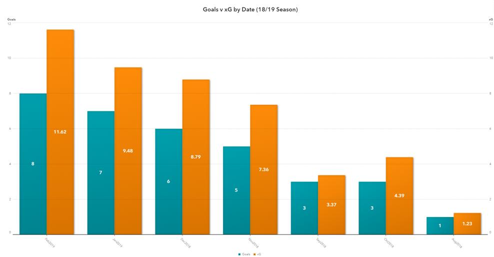
The xG metric suggests that a trend like this isn’t sustainable over a long period, despite its persistence through a 38-game season. If we have a look at this season’s numbers so far (below), we see the reverse is true. So the effect of combining this with last season (and extending the sample size) is that that we revert more to the norm of xG equals actual goals.
Limitations
Expected goals has the potential to completely revolutionise analytics in football. It can open a whole new world where data can now tell a story, beyond just reporting on the game. And it will only get better as more data about shots creates more accurate models. However, it doesn’t come without limitations.
Scoring goals is a skill. And while one could rightfully argue that getting into scoring positions is more important than the finish, it’s still possible for one player to be better than others at putting the ball in the back of the net. The xG metric doesn’t consider this, and it needs to be put in context.
Anyone who’s ever watched or played football knows that it is the most open game with more unique possibilities than any other sport. This could also be a reason why it’s behind on useful analytics compared to other team sports. But it also means that only accommodating several variables (shot type, location, angle, etc.) does not tell the full story. There are countless variables we fail to consider when calculating expected goals, and perhaps we will never be able to fully or accurately calculate them.
Anyone who’s ever watched or played football knows that it is the most open game with more unique possibilities than any other sport. Click To TweetFinally, there is the human factor. Players who "underperform" could have their confidence suffer due to lack of goals, which may genuinely dry up their output over the long run. Similarly, an overperforming run could boost someone’s confidence, fostering continuous improvement.
The xG metric is a great starting point, but as with all other statistics, it requires context. For example, if you look in more detail at the chances taken and chances missed by an individual player, you may find out why the player scores in some situations but not in others.
The future of analytics in football
Despite limitations, football looks like it will catch up with the rest of the sporting world in terms of analytics. The xG metric will allow us to scout up-and-coming players to see if they’re overperforming or the real deal. Teams can alter tactics to focus on chance creation over the long run as opposed to focusing purely on the next result. And finally, it will allow us to open a new chapter in football analytics, where the use of AI can play a valuable role, as it’s already doing with SciSports. The Dutch sports analytics company gives a quality rating to each individual player using model-based mathematical algorithms, based on the contribution of a player to the team's result, all in real time.
In my next post, I will dive deeper into statistical concepts regarding xG. I will explore how efficient it is in predicting both short- and long-term results and compare it to other metrics.

3 Comments
Haidar, interesting line of discovery. How do you calculate xG?
Thanks Chaz! xG is calculated by using historic data of similar shots being taken in the past, and how likely they have resulted in a goal.
For example, if 10 different players had taken a shot from the edge the box, from open play, with their right foot and was assisted by another player and 2 have been scored - this type of shot would have an xG of 0.2. If we use the same sample but the but 10 yards further back, it might be 1 of 10 shots (0.1xG).
Over a large sample size this becomes more accurate - hope that explains it?
Great post Haidar, thanks for writing it up! Looking forward to your next one!