Here in the US, there's a lot of talk about the flu each year. First, people discuss whether or not to get the flu shot. Then there are discussions about whether or not you or your friends have the flu (or something else). Then the discussions about what strain of flu is going around - is it the strain the shots were designed to protect against, or some other strain? It's difficult to get definitive data about cases of the flu since not every case is reported. And whereas not every illness is reported, all deaths are reported ... and therefore the number of deaths attributed to the flu is probably a somewhat comparable metric from year to year. So let's plot the data.
CDC's Flu Deaths graph
First I did a bit of searching for possible data sources, and looked to see if there might already be some graphs. I found some plots on the Centers for Disease Control (CDC) website that were close to what I was looking for. But this graph contains both influenza (flu) and pneumonia, whereas I was looking for just the flu. Also, it showed the % of deaths, whereas I was more interested in the total number of deaths. And, since my brain doesn't really think in "week numbers" (52 weeks per year), the bottom axis of the graph didn't make much sense to me. And their graph only went through the end of 2018.
My Graph (2019)
Since that graph wasn't quite what I was looking for, I decided to download the raw data and create my own graph ... I wanted to include the latest data (to see what the numbers were doing in 2019), and I wanted to make my graph easier to understand. The data is reported by year and week, therefore it's a pretty simple matter to create a plot for one year - here's how to plot the current year (2019). Note that rather than using a line plot like the original graph, I start my y-axis at zero and shade the area under the line. Also, I'm plotting the number of deaths attributed to the flu, rather than the percent of deaths attributed to the flu & pneumonia.
title1 h=14pt c=gray33 "Influenza (Flu) Deaths Per Week in the US in 2019";
proc sgplot data=my_data (where=(year=2019));
band x=week lower=0 upper=flu_deaths / fill fillattrs=(color=red);
yaxis values=(0 to 400 by 100);
xaxis values=(1 to 52 by 1) valueattrs=(size=6pt);
run;
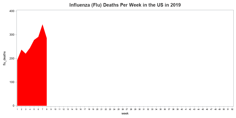
Well, that's the 2019 data! ... But is ~300 deaths per week better or worse than usual? Let's plot some other years of data, so we have something to compare the 2019 values to!
My Graph (10 years)
When you have your time stored in two separate variables (year & week), it's a bit tricky to plot more than one year on the same plot. One way you could do it would be to create a new variable that combines the year and week (as year + 1/52 for each week), and plot that new variable on a continuous axis. Another way would be to create a separate plot for each year (using a 'by year' statement) - then you would have a bunch of small multiples to compare. But I chose a slightly different approach ... I used Proc SGPanel to create a separate graph for each year, but 'panel' them together so that they appear to be one continuous graph, sharing a response axis.
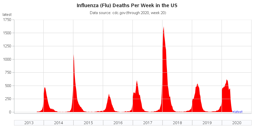
title1 h=14pt c=gray33 "Influenza (Flu) Deaths Per Week in the US";
proc sgpanel data=my_data noautolegend;
format flu_deaths latest comma10.0;
panelby year / onepanel columns=10 novarname
colheaderpos=bottom layout=columnlattice
headerattrs=(size=12pt color=gray33) noborder;
band x=week lower=0 upper=flu_deaths / fill fillattrs=(color=red)
tip=(flu_deaths year week);
rowaxis labelpos=top values=(0 to 1750 by 250)
valueattrs=(size=11pt color=gray33)
label='Deaths' labelattrs=(size=11pt color=gray33)
offsetmax=0 offsetmin=0;
colaxis values=(1 to 52 by 1) display=(nolabel noticks novalues)
offsetmax=0 offsetmin=0;
refline 52 / axis=x lineattrs=(color=graycc thickness=1px);
refline 0 to 1750 by 250 / axis=y lineattrs=(color=graycc thickness=1px);
run;
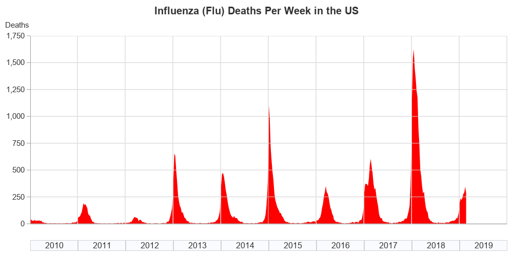
Now that we have ~10 years of data to compare, we can see that last year (2018) had a relatively high number of flu deaths, but this year seems to be much lower (keep your fingers crossed, because this year's flu season isn't over yet!) Speaking of this year's flu season not being over, it's a little difficult to tell exactly how far into this year the graph & data go. And was the final 2019 data point at the 'peak' of the graph, or has the number of deaths started to drop (below the peak)? Let's customize the graph to make these things a little more evident.
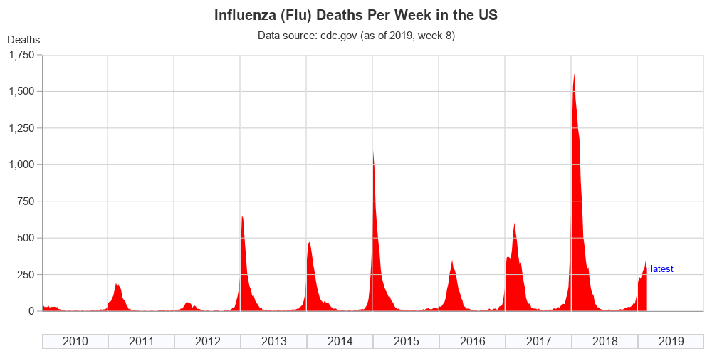
My Graph (customized)
First, I determined the most recent year & week in the data, and added an extra variable to the dataset such that only that particular week had a value. I then added a scatter plot marker (blue circle) at that value, and labeled it as 'latest'.
proc sort data=my_data out=my_data;
by year week;
run;
data my_data; set my_data end=last;
if last then do;
latest=flu_deaths;
latest_text='latest';
end;
run;
scatter x=week y=latest / markerattrs=(color=blue symbol=circle)
datalabel=latest_text datalabelpos=right
datalabelattrs=(color=blue size=10pt);
And then I took those values for the most recent year & week, and stored them as macro variables, so I could easily show them in the title.
proc sql noprint;
select year into :maxyear separated by ' ' from my_data where latest^=.;
select week into :maxweek separated by ' ' from my_data where latest^=.;
quit; run;
title2 h=12pt c=gray99 ls=0.5 "Data source: cdc.gov (&maxyear, week &maxweek snapshot)";
But there was one other user-friendly thing I wanted to do. I wanted the user to be able to click the 'Data source:' text, and have it link to the actual data. The link= option for titles in ODS Graphics hasn't been implemented yet, so I had to annotate the 'Data source:' text, rather than using a title statement.
data anno_title2;
length label $100 anchor x1space y1space function $50 textcolor $12;
function='text';
x1=50; y1=90;
x1space='graphpercent'; y1space='graphpercent';
anchor='center';
textcolor="gray33"; textsize=11; textweight='normal';
width=100; widthunit='percent';
url="https://www.cdc.gov/flu/weekly/weeklyarchives2018-2019/data/NCHSData09.csv";
label="Data source: cdc.gov (as of &maxyear, week &maxweek)"; output;
run;
Now we have a graph that allows the user to easily compare the current year to previous years, see multiple visual cues that tell what is the last data point on the graph, and click the 'Data source:' text in the title to download the actual data. (click the image below to see the interactive version with the drill-down to the data)
What is your flu prediction for the rest of this season - are we past the peak, or will the number of deaths per week continue to rise? What features do you like, or not like about this graph? What suggestions do you have for improving it?
(For the programmers out there, here's a link to the SAS code.)
LEARN MORE | You might also be interested in our Coronavirus blog posts
July 2019 Update:
Now that the flu season is over, here's a link to my latest/updated graph:


18 Comments
Hi Robert,
Your SAS Graphs is a treasure trove of Knowledge for SAS Programmers like me. Do you mind telling me where I can find the entire SAS code for the above Topic? I usually manage to locate them at your website : http://robslink.com/SAS/Home.htm . But i could not find this one.
Thanks.
I have just now added a link to the code, at the bottom of the blog... https://blogs.sas.com/content/graphicallyspeaking/files/2019/03/us_flu_deaths.txt
Thanks, Robert for your Prompt reply. Please continue sharing your great graphs with us and also including the link to SAS code when possible (just a small suggestion).
It’s nice to see The Graph Guy starting to use ODS Graphics!
Hi Robert, very nice and informative graph. I like the link to the actual data. The panel approach is a smart solution to solve plotting two time variables. Thanks
Glad you like the link to the data!
So often these days, I see some 'random' claim on social media about some data/numbers that would purportedly back up the point a person is making ... but they seldom have a link to the source of the data. Hopefully I can start a trend (at least in graphs) of always providing a link to the data source! 🙂
Do we have a flu chart for the last 100 years.
What would be interesting is to compare the 1918 flu with current covud trends to predict how/ when covid would be less aggressive such as the flu. After 1920 1% of the world was not dying of flu every year...
Regardless of how the x axis is labeled, for me a relevant and insight-providing way to present the data, whatever is used to measure impact of flu, would be to somehow stack the seasonal years (defined as,say July 1 to June 30). I want to see to what extent the peaks nearly coincide, and to compare the trends, not just their peaks. There are at least two ways to do thus: (a) an overlay plot; and (b) a one-column panel, where, if possible, each plot in the panel uses a range specific to its maximum.
How about a graph on measles? Including deaths/ages?
Love reading your blogs! I learn SAS and something about the world I wouldn't know to ask.
Great minds think alike! ... After hearing that the measles was on the rise again, I was just getting ready to try to find some data to plot! 🙂
Why not update in this time ?
Here's a more recent blog post, with a similar graph that's more up-to-date:
https://blogs.sas.com/content/graphicallyspeaking/2020/01/23/how-to-prepare-your-graphs-for-flu-season/
Please update with covid-19
How about a comparison of the weekly deaths from Covid-19 and the weekly deaths from the flu (from 2018 & 2019)? And with a note for Total Deaths for those years & Covid-19 (2020).
I second this request.
Hi Robert, Thanks for the concise graphs. Would you consider creating graph for Covid19 by city with overlay of 5g implementation? No one has created this graph yet, and it would sure be nice to have a factually based visual. I'm a "word" girl gathering data, but creating a graph is out of my league.
That could be an interesting graph, but I don't have access to data at the city level. 🙂
An interesting experiment (to eliminate all variables) might be a graph of ALL deaths.