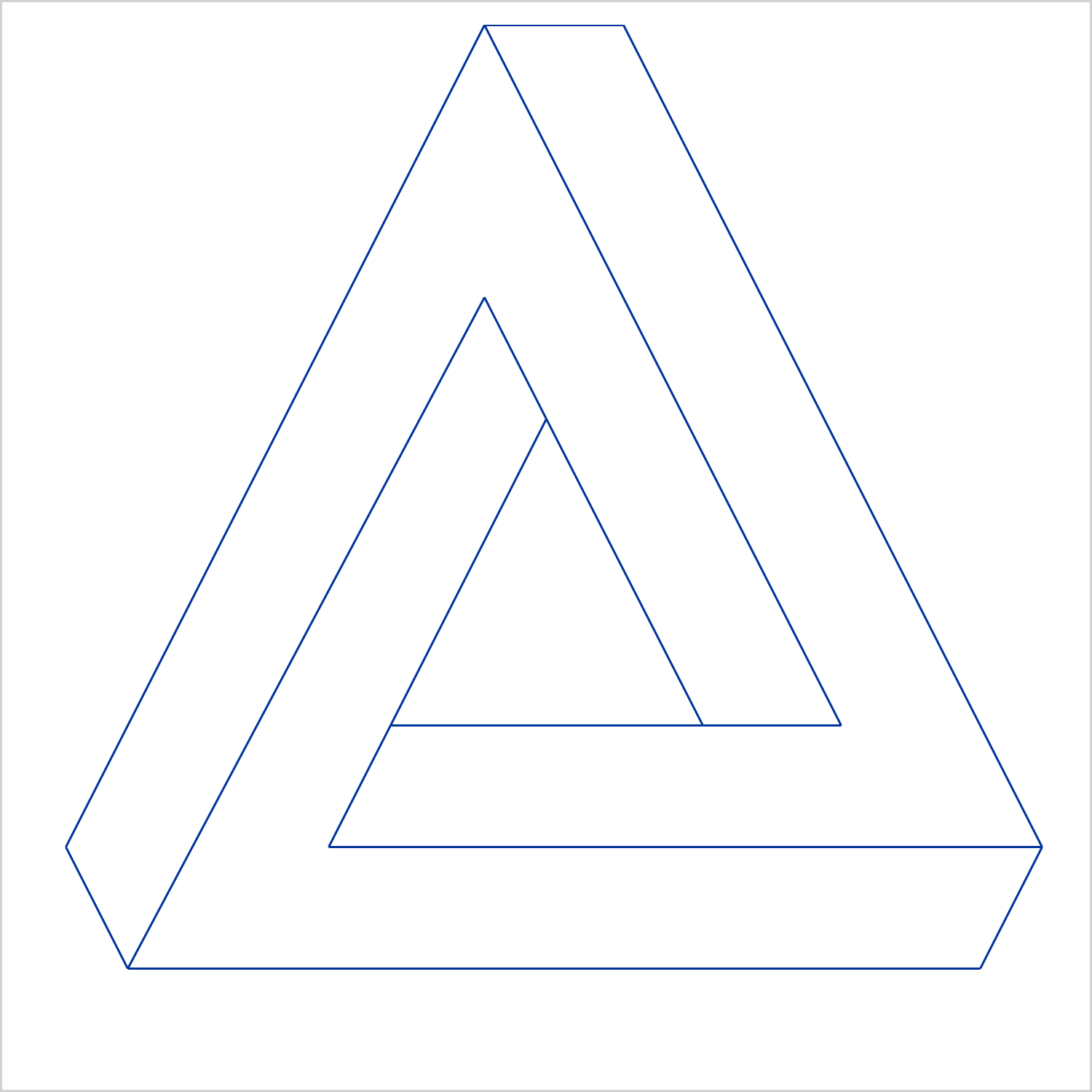
I hope everyone has noticed some new shortcuts in Graphically Speaking. As you scroll down and look to the right, there are shortcuts for Sanjay's getting started and clinical graphs posts and one for my advanced blogs. When Sanjay asked me to make an icon for my advanced blogs, at first I had no idea what to do. I eventually thought of making an impossible triangle (Penrose triangle). I put together something ad hoc but then wondered about the best way to draw an impossible triangle. I will share ways to draw, erase, fill, and rotate it. While you will probably never need to draw a Penrose shape, you might find some of the techniques that I use to be handy in other applications.

Using Method 2, Extending a Triangle, I wrote the following step that generates the coordinates for the 15 line segments, from (xo, yo) to (x, y).
* Draw 15 sides;
data x(keep=x y xo yo);
   e = 4; r = 4.5; c = 0; z = 0;
   b = sqrt((e ** 2) / 5);
   a = 2 * b;
   h = 2 * r;

   xo = c - r;     yo = z;     x = c + r;  y = z;      output;
   xo = c + r;     yo = z;     x = c;      y = h;      output;
   xo = c;         yo = h;     x = c - r;  y = z;      output;

   xo = c + r;     yo = z;     x = xo + e; y = yo;     output;
   xo = c;         yo = h;     x = c - b;  y = h + a;  output;
   xo = c - r;     yo = z;     x = xo - b; y = yo - a; output;

   xo = c + r + e; yo = z;     x7 = c - b;
                               y7 = 2 * (r + e + b) - yo; x = x7; y = y7; output;
   xo = c     - b; yo = h + a; x8 = c - r - 2 * b - e;
                               y8 = z - 2 * a;            x = x8; y = y8; output;
   xo = c - r - b; yo = z - a; x9 = c + r + b + 2 * e;
                               y9 = yo;                   x = x9; y = y9; output;

   xo = x9; yo = y9; x10 = xo - b; y10 = yo - a; x = x10; y = y10; output;
   xo = x7; yo = y7; x11 = xo + e; y11 = yo;     x = x11; y = y11; output;
   xo = x8; yo = y8; x12 = xo - b; y12 = yo + a; x = x12; y = y12; output;

   xo = x11; yo = y11; x = x9; y = y9; output;
   xo = x12; yo = y12; x = x7; y = y7; output;
   xo = x10; yo = y10; x = x8; y = y8; output;
run; |
My geometry is a bit rusty, so there might be easier ways, but this worked. The following step uses a VECTOR statement to draw the shape.
ods graphics on / height=5in width=5in; * Draw the shape; proc sgplot data=x noautolegend noborder aspect=1; vector x=x y=y / xorigin=xo yorigin=yo noarrowheads; xaxis display=none offsetmin=0 offsetmax=0; yaxis display=none offsetmin=0 offsetmax=0; run; |
As I continued to play with this shape, I found it helpful to label each segment with the order in which it is drawn.
* Add segment number; data x2; set x; g + 1; run; * Draw the shape along with the side numbers; proc sgplot data=x2 noautolegend noborder aspect=1; vector x=x y=y / xorigin=xo yorigin=yo noarrowheads datalabel=g group=g; xaxis display=none offsetmin=0 offsetmax=0; yaxis display=none offsetmin=0 offsetmax=0; run; |
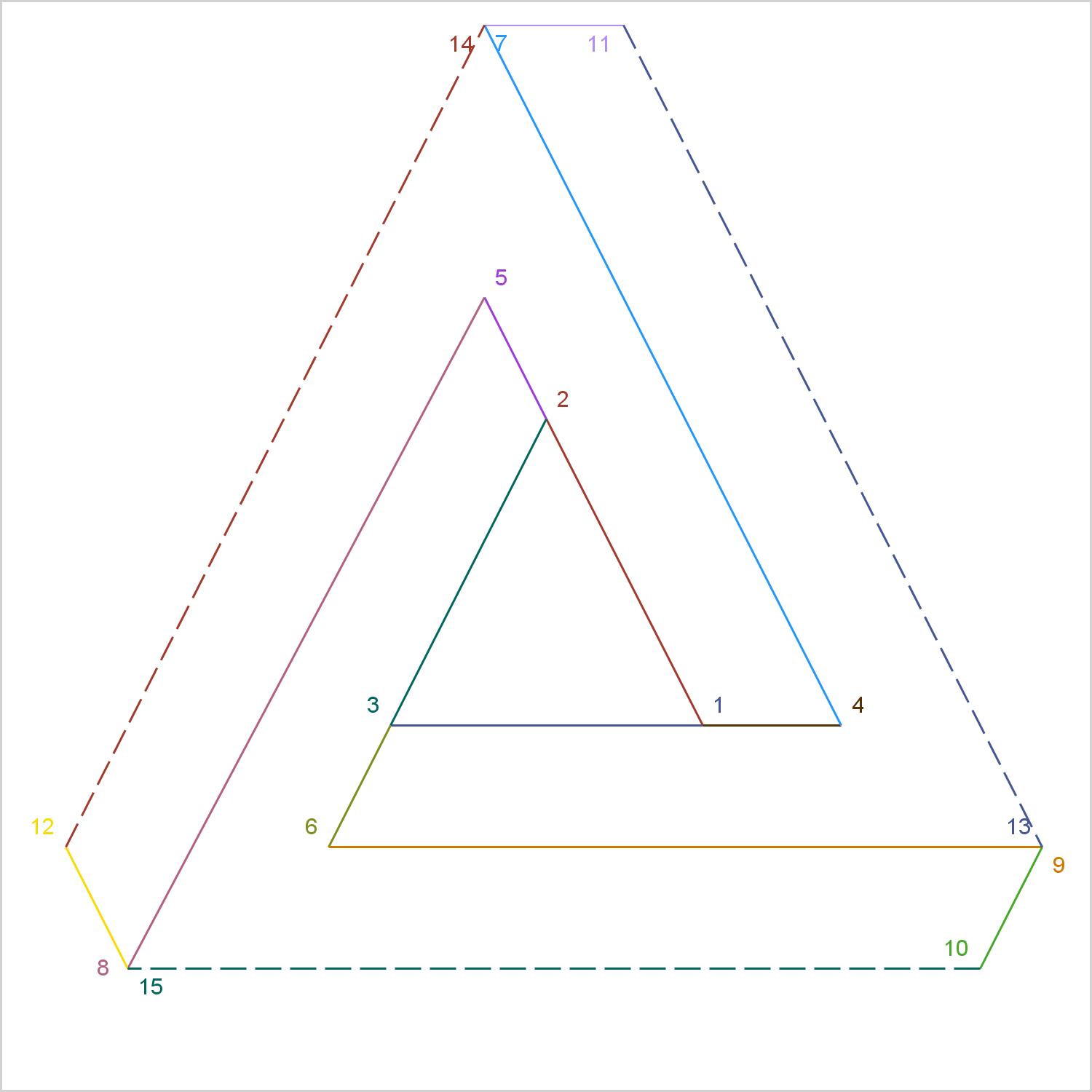
The last three lines are dashed and the colors of those lines match the colors of the first three lines. This is because of the default ATTRPRIORITY=COLOR specification in the HTMLBlue style.
While I used the method of extending a triangle, you can also draw the shape by drawing three polygons. The following step creates three polygons from the relevant seven sides in the X data set.
* Convert to polygons;
data x4(keep=g x y);
   g = 1;
   i = 1;
   set x point=i; x = xo; y = yo; output;
   do i = 1, 4, 7, 11, 13, 9, 6;
      hx = x; hy = y;
      set x point=i;
      if abs(y - hy) le 1e-6 and abs(x - hx) le 1e-6 then do; x = xo; y = yo; end;
      output;
   end;

   g = 2;
   i = 10;
   set x point=i; x = xo; y = yo; output;
   do i = 10, 15, 8, 5, 3, 6, 9;
      hx = x; hy = y;
      set x point=i;
      if abs(y - hy) le 1e-6 and abs(x - hx) le 1e-6 then do; x = xo; y = yo; end;
      output;
   end;

   g = 3;
   i = 4;
   set x point=i; x = xo; y = yo; output;
   do i = 4, 7, 14, 12, 8, 5, 2;
      hx = x; hy = y;
      set x point=i;
      if abs(y - hy) le 1e-6 and abs(x - hx) le 1e-6 then do; x = xo; y = yo; end;
      output;
   end;
   stop;
run; |
The STOP statement is required when none of the SET statements attempts to read a record beyond the end of the file. When the end of file is not hit, the DATA step executes again unless you use a STOP statement to stop it. This DATA step is an infinite loop without the STOP statement.
The vector version of the plot uses two points per observation, the options X=X, Y=Y, XORIGIN=XO, and YORIGIN=YO, and a data set that has 15 observations (one for each line segment). The polygon version uses one point per observation, the options X=X and Y=Y, and a data set that has 15 observations (eight points per polygon including one starting point and seven continuations). The IF statement replaces X and Y by XO and YO when X and Y match the previous point. The following step creates the impossible triangle from the three polygons.
proc sgplot data=x4 noautolegend noborder aspect=1; polygon x=x y=y id=g / group=g fill dataskin=gloss; xaxis display=none offsetmin=0 offsetmax=0; yaxis display=none offsetmin=0 offsetmax=0; run; |

Now returning to the original data set, you can output multiple copies of the triangle, each a rotation of the previous version, by using PROC IML and rotation matrices.
* Rotate the shape;
proc iml;
   use x; read all into x;
   x1 = x[,1:2];
   x2 = x[,3:4];

   do t = 0 to 2 * constant('pi') by constant('pi') / 8;
      r = (cos(t) || -sin(t)) //
          (sin(t) ||  cos(t));
      o1 = o1 // x1 * r;
      o2 = o2 // x2 * r;
   end;
   x = o1 || o2;
   create r from x[colname={'xo' 'yo' 'x' 'y'}]; append from x;
quit; |
The PROC IML step rotates the shape 0 radians, π / 8 radians, and so on until it reaches a complete rotation of 2π radians.
You can also randomly sort the line segments.
* Randomly sort the sides for construction and removal; data r2; set x; r1 = uniform(513); r2 = uniform(513); run; proc sort data=r2 out=r3; by r1; run; proc sort data=r2 out=r4; by r2; run; |
The following creates a data set that has a BY variable that draws the shape by extending a triangle, rotates it, removes it, draws it as three polygons, removes it a different way, generates the segments in random order, then randomly removes them. The BY variable G changes values for each step, but the same value is used in multiple steps.
data x3;
   * Draw the shape by extending a triangle;
   do g = 1 to 15;
      do i = 1 to g;
         set x point=i;
         output;
      end;
   end;
   * Rotate it;
   do g = 1 to 17;
      do i = 1 to 15;
         r + 1;
         set r point=r;
         output;
      end;
   end;
   * Remove it;
   do g = 1 to 15;
      do i = g to 15;
         set x point=i;
         output;
      end;
   end;
   * Gone, blank;
   g = 0; call missing(x, y, xo, yo); output;
   * Draw the shape by drawing three polygons;
   array z[15] _temporary_ (1 4 7 11 13 9 6 10 15 8 5 3 2 14 12);
   do g = 1 to dim(z);
      do i = 1 to g;
         j = z[i];
         set x point=j;
         output;
      end;
   end;
   * Remove it;
   do g = 1 to 15;
      do i = 1 to 16 - g;
         set x point=i;
         output;
      end;
   end;
   * Gone, blank;
   g = 0; call missing(x, y, xo, yo); output;
   * Randomly draw the shape;
   do g = 1 to 15;
      do i = 1 to g;
         set r3 point=i;
         output;
      end;
   end;
   * Randomly remove the shape;
   do g = 1 to 15;
      do i = 1 to 16 - g;
         set r4 point=i;
         output;
      end;
   end;
   * Gone, blank;
   g = 0; call missing(x, y, xo, yo); output;
   stop;
run; |
The following steps display in an animated file the filled triangle and the versions from the preceding DATA step.
ods _all_ close;
options papersize=('5in', '5in') printerpath=gif animation=start
        animduration=.5 animloop=yes noanimoverlay nobyline nonumber;
ods printer file='triangle.gif';

ods graphics / width=5in height=5in dataskinmax=100000 groupmax=100000
               antialiasmax=100000;

proc sgplot data=x4 noautolegend noborder aspect=1;
   polygon x=x y=y id=g / group=g fill dataskin=gloss;
   xaxis display=none offsetmin=0 offsetmax=0 values=(-23 23);
   yaxis display=none offsetmin=0 offsetmax=0 values=(-23 23);
run;

proc sgplot data=x3 noautolegend noborder aspect=1 nowall;
   vector x=x y=y / xorigin=xo yorigin=yo noarrowheads;
   xaxis display=none offsetmin=0 offsetmax=0 values=(-23 23);
   yaxis display=none offsetmin=0 offsetmax=0 values=(-23 23);
   by notsorted g;
run;

proc sgplot data=x4 noautolegend noborder aspect=1;
   polygon x=x y=y id=g / group=g fill dataskin=gloss;
   xaxis display=none offsetmin=0 offsetmax=0 values=(-23 23);
   yaxis display=none offsetmin=0 offsetmax=0 values=(-23 23);
run;

options printerpath=gif animation=stop;
ods printer close; |
The results are displayed at the top of the blog. Clearly, there is more than just fun and games going on here. Drawing and rotating the triangle requires basic geometry and trigonometry. Several useful data set manipulations are used including the POINT= option in the SET statement. Since BY variables do not always increase or decrease, you need the NOTSORTED option in the BY statement. Each triangle, including the rotations, must appear in a consistent part of the graph. This is accomplished by ensuring that each graph is anchored by two corner points: (-23, -23) and (23, 23). These are specified as extreme tick values, but they are not displayed. You can apply the techniques that I used here if you want to display step-by-step instructions, if you need to rotate the coordinates for a shape, or if you just want to have fun with ODS Graphics.
