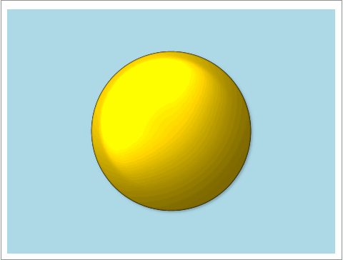
In Sanjay's previous post, Fun with ODS Graphics: Eclipse animation, he showed a very cool method of making an animated gif file by using PROC SGPLOT. At the end, he added: "One additional feature could be to simulate the corona during the full eclipse. Any thoughts?" I took the bait. I wanted to share the result, not because of my attempt at making a corona, but because it provides a nice illustration of range attribute maps, colors versus "alt" colors, DATA step programming, PROC SGPLOT, and assorted options.
I never made an animated gif file before, so I was excited to try. I found that if you know how to create a graph with BY groups and you can copy a few additional statements and options, then you know enough to make one. All you need to do is make a progression of graphs where each BY group displays the next frame in the animation.
I decided to go a bit beyond Sanjay's example in a few ways. I wanted my range attribute map to be a bit more granular and animate the sky from light blue to gray to black. I wanted the color changes to be aligned with the relative positions of the sun and moon. Furthermore, at the same time that the sky is changing, I wanted stars to go from light blue (invisible) to gray (still invisible) to yellow (visible when the background is black). This requires creating two coordinated range attribute maps. As I developed the code, I wanted as much as possible to programatically create the attribute map and not type anything into the data set that I could create from other parts of the data set. (This makes life easier when you are repeatedly fiddling with the ranges and colors.) I created two range attribute maps in one data set. Each specified the same range of frames in the Min and Max variables. The first (ID='sky') varied the colors for the sky, which is created by a POLYGON statement, using the variables ColorModel1 and ColorModel2, which are the variables for fill colors. The second (ID='star') varied the colors for the star, which are created by a SCATTER statement, using the variables AltColorModel1 and AltColorModel2, which are the variables for marker and line colors. The range attribute map data set is as follows:
id min max colormodel1 colormodel2 altcolormodel1 altcolormodel2 sky 1 20 lightblue lightblue sky 21 35 lightblue gray sky 36 41 gray black sky 42 46 black black sky 47 52 black gray sky 53 67 gray lightblue sky 68 90 lightblue lightblue star 1 20 lightblue lightblue star 21 35 lightblue gray star 36 41 gray yellow star 42 46 yellow yellow star 47 52 yellow gray star 53 67 gray lightblue star 68 90 lightblue lightblue |
The first row keeps the colors a constant light blue for slides 1 to 20. Then the colors range to gray, black and light blue across subsequent observations. I generated it in the following steps:
data mymap;
   retain id "sky ";
   length min max 8 colormodel1 colormodel2 $ 12;
   input max colormodel2;
   colormodel1 = lag(colormodel2);
   if colormodel1 eq ' ' then colormodel1 = colormodel2;
   min = sum(lag(max), 1);
   datalines;
20 lightblue
35 gray
41 black
46 black
52 gray
67 lightblue
90 lightblue
;

data myrattrmap;
   set mymap mymap(in=i);
   if i then do;
      id = 'star';
      altcolormodel1 = ifc(colormodel1 = 'black', 'yellow', colormodel1);
      altcolormodel2 = ifc(colormodel2 = 'black', 'yellow', colormodel2);
      call missing(colormodel1,colormodel2);
   end;
run; |
The instream data has only one color variable, ColorModel2. The first color, ColorModel1, is a simple function of the lag of ColorModel2. Then the colors in the second map can easily be created from the colors in the first map. Similarly, Min is created from Max by using a single assignment statement.
The POLYGON statement uses the options COLORRESPONSE=SKYID and RATTRID=SKY to make it aware of the range attribute map specifications. The variable SkyID is in the DATA=ECLIPSE data set and matches the Frame variable, which is the BY variable. The SCATTER statement uses the options COLORRESPONSE=FRAME and RATTRID=STAR to make it aware of the range attribute map specifications. The PROC STATEMENT names the range attribute map in the RATTRMAP=MYRATTRMAP option. The values of the the Min and Max variables in the range attribute map data set correspond to the values of SkyID and Frame variables in the DATA= data set. The DATA=ECLIPSE data set is large. Each frame has at least 158 observations. There are 151 stars whose coordinates are in the variables StX and StY. Here are 3 of them.
moon cx cy g frame stx sty sunX sunY sz moonX Y skyid x y 0.5 0.5 0 1 0.23611 0.88923 . . . . . . . . 0.5 0.5 0 1 0.58173 0.97746 . . . . . . . . 0.5 0.5 0 1 0.84667 0.80484 . . . . . . . . |
The position of the sun comes next, followed by the position of the moon, followed by the coordinates for the sky.
moon cx cy g frame stx sty sunX sunY sz moonX Y skyid x y 0.5 0.5 0 1 . . 0.5 0.5 50 . . . . . 0.5 0.5 0 1 . . . . 49 1.275 0.5 . . . 0.5 0.5 0 1 . . . . 1 . . 1 0 -1 0.5 0.5 0 1 . . . . 1 . . 1 1 -1 0.5 0.5 0 1 . . . . 1 . . 1 1 1 0.5 0.5 0 1 . . . . 1 . . 1 0 1 |
This is repeated for each frame, adjusting the values as needed. The variables CX and CY provide coordinates for the corona. These are filled in later.
Someone more artistic than I am could no doubt find a better way to represent the corona. I generated random points from three bivariate normal distributions and displayed functions of them as vectors. Rick Wicklin's post How to generate multiple samples from the multivariate normal distribution in SAS provides the method that I used to generate the bivariate normal variables. Here are the coordinates of the first few vectors.
cx cy 0.54229 0.78054 0.44437 0.24627 0.73190 0.80161 0.29754 0.19227 0.73628 0.62001 |
Then I use a DATA step read the original data and in frames 41 through 48 replaced the place-holder coordinates with the vector coordinates. They were slightly changed in each frame to add a twinkle.
This is the final step that makes the graph.
ods _all_ close;
options papersize=('5 in', '3.8 in') printerpath=gif animation=start
        animduration=.1 animloop=yes noanimoverlay nobyline nonumber;
ods printer file='Eclipse.gif';

ods graphics / width=4.9895in height=3.7999in dataskinmax=100000 groupmax=100000
               antialiasmax=100000 attrpriority=none;
proc sgplot data=eclipse2 noautolegend noborder nowall rattrmap=myrattrmap;
   styleattrs datalinepatterns=(solid) datacontrastcolors=(white);
   by frame;
   polygon id=skyid x=x y=y / colorresponse=skyid fill nooutline rattrid=sky;
   scatter x=stx y=sty /   rattrid=star colorresponse=frame
                           markerattrs=(symbol=starfilled size=3px);
   vector  x=cx  y=cy  /   lineattrs=(pattern=1 color=cxdddddd thickness=3px)
                           noarrowheads xorigin=.5 yorigin=.5;
   bubble x=sunX  y=sunY   size=sz / colormodel=(yelloworange) colorresponse=sunX dataskin=sheen bradiusmax=120;
   bubble x=moonX y=moonY  size=sz / colormodel=(black) colorresponse=moonX dataskin=sheen bradiusmax=120;
   yaxis display=none min=0 max=1 offsetmin=0 offsetmax=0;
   xaxis display=none min=0 max=1 offsetmin=0 offsetmax=0;
run;

options printerpath=gif animation=stop;
ods printer close; |
It creates a file Eclipse.gif in the PRINTER destination. The options ANIMATION=START, ANIMDURATION=.1, ANIMLOOP=YES, and NOANIMOVERLAY create the animation. As I developed the code, I often used ANIMDURATION=.5 so that I could get a longer look at each frame. I set some MAX= options to enable options that get disabled as the graph gets bigger. I also created a graph that just fit inside the specified graph size ("paper size") and disabled BY lines and page numbers (NOBYLINE and NONUMBER).
In the POLYGON statement which creates the sky, the coordinates change in each frame and the range attribute map controls the colors. In the SCATTER statement which creates the stars, the coordinates stay the same in each frame and the range attribute map controls the colors. If you were interested in making a smaller data set, you could only create all of the stars when they are visible (as I did with the corona). In the VECTOR statement which creates the stars, the coordinates slightly vary in each corona frame and the range attribute map is not used. Since there are so many vectors, other frames have place-holder coordinates rather than all of the vector coordinates. The two BUBBLE statements create the sun and moon. Coordinates vary, and these two statements do not use either range attribute map.
While you might never need to make an animated gif, there are still many useful techniques that are illustrated in this example. There are some interesting DATA step techniques including creating a data set using the DATA step and then replacing part of it using another DATA step and the POINT= option in the SET statement. Attribute maps are one of my favorite techniques in ODS Graphics. Usually, I have only needed one in any particular graph. This problem provides a nice illustration that you can use more than one and that you can coordinate them. Finally, if you have a way of making a more realistic corona, I would love to see it!
Update August 28, 2017.
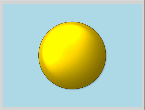
Sanjay pointed out that it would have been more accurate if I had made the moon invisible as it crosses the sky. This means I need to create three partitions in my range attribute map (one each for the sky, stars, and moon), and I need to coordinate the sky and moon colors. In this version, I also make a geometric shape for the corona. It is still unsatisfactory. I think you would need to trace out an actual corona and store a set of edge coordinates to come up with something more satisfactory.


2 Comments
Nicely done Warren!
Thanks, Kirk!