The Scatter Plot Matrix is a great tool that provides a quick visual of potential associations between variables. This may provide the analyst some hints on how to proceed with the analysis.
Matrix of lab values for liver function tests are commonly used in clinical research. The SGSCATTER procedure provides an easy way to create matrix graphs as shown below. Click on the images for higher resolution image.
3x3 Matrix view of lab values:
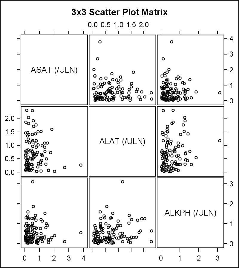
Proc SGSCATTER Code:
title '3x3 Scatter Plot Matrix'; ods graphics / reset width=4in height=4.5in imagename='Matrix_3x3'; proc sgscatter data=safety; matrix asat alat alkph; run; |
4x4 Matrix view of lab values with distribution plots:
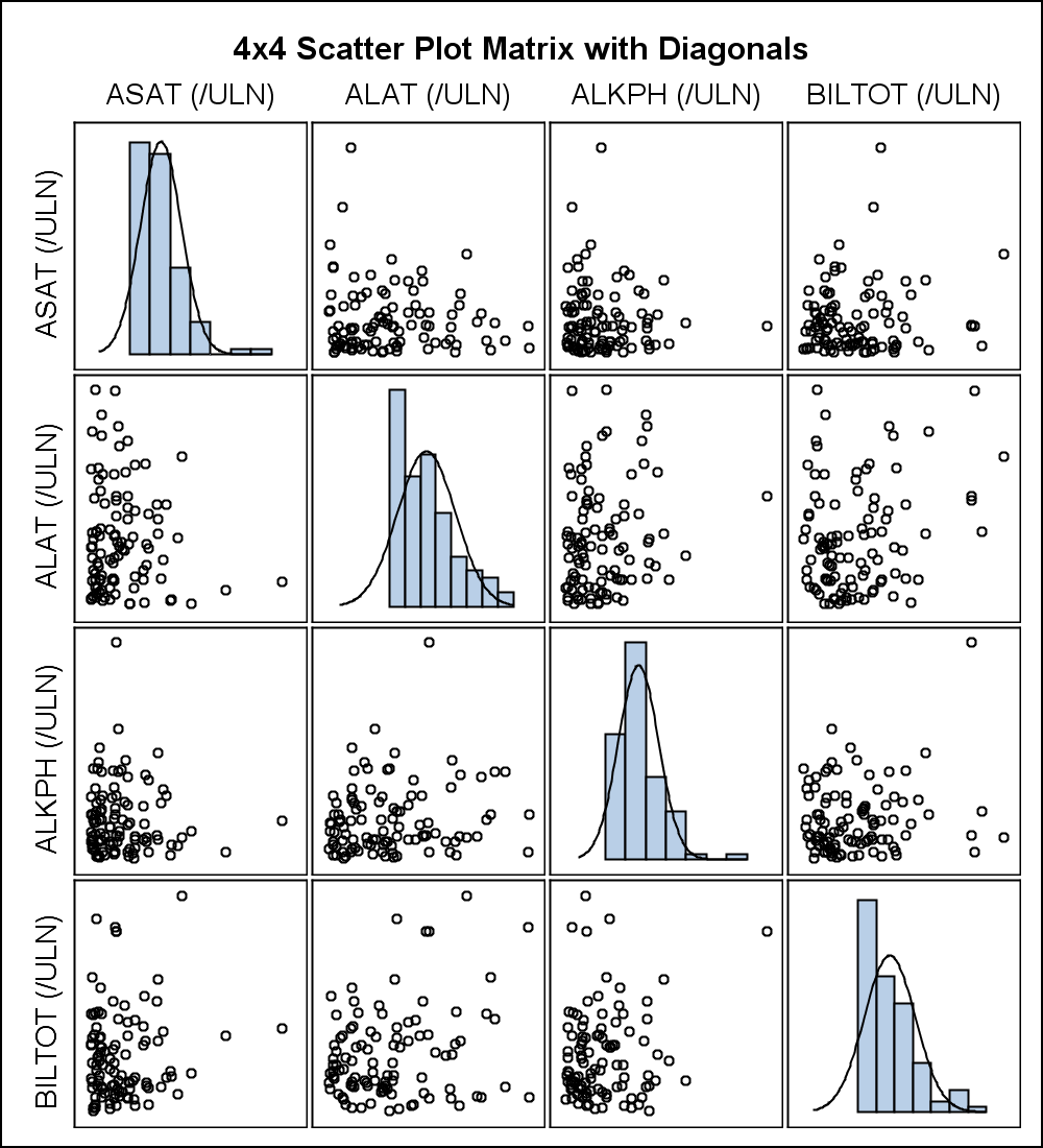
Proc SGSCATTER Code:
title '4x4 Scatter Plot Matrix with Diagonals'; ods graphics / reset width=5in height=5.5in imagename='Matrix_4x4_Diag'; proc sgscatter data=safety; matrix asat alat alkph biltot / diagonal=(histogram normal); run; |
There are a few issues with these graphs from a clinical perspective.
- The matrix statement does not provide any way to customize the axes.
- There is no way to indicate the clinical concern levels in the graphs.
- The upper triangle of the matrix is a mirror image of the lower triangle, and hence wasteful of the space.
A closer examination of the graph indicates that we can eliminate the top row and right column of the matrix, to get a smaller 3x3 arrangement of the 4 variables, and still have all the pairwise scatterplot combinations for all the variables. In fact, this arrangement is popular in the clinical domain as shown below in what can be called the "Compact Matrix".
Compact Matrix for 4 variables:
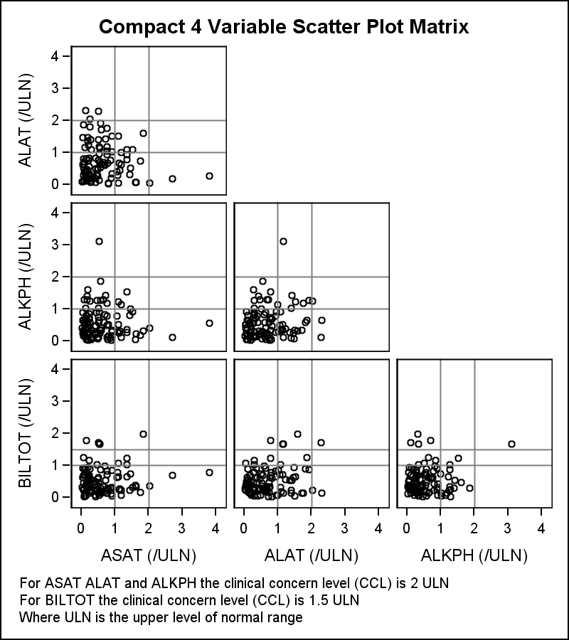
This matrix has the following features:
- All six pairwise combinations of the four variables are included in the graph.
- The matrix occupies only a 3x3 grid for 4 variables hence uses the space more efficiently.
- Drawing of the upper triangle is eliminated resulting in a cleaner, uncluttered graph.
- Axes are customized.
- Clinical concern levels are indicated by test case.
Given that this arrangement is very popular, we will likely include an option to draw compact matrices in the next release based on the work shown here. But how do we do this now?
For SAS 9.2 and SAS 9.3, the ScatterPlotMatrix both in GTL and SGSCATTER already use the LAYOUT LATTICE in GTL to create this graph. So, it is possible to write a macro to draw a "CompactMatrix" using the lattice layout, axis options and reference lines in GTL to create this graph.
Macro invocation for 4-variable Compact Matrix:
%CompactMatrixMacro(data=safety, var1=asat, var2=alat, var3=alkph, var4=biltot, title=Compact 4 Variable Scatter Plot Matrix, footnote=For ASAT ALAT and ALKPH the clinical concern level (CCL) is 2 ULN, footnote2=For BILTOT the clinical concern level (CCL) is 1.5 ULN, footnote3=Where ULN is the upper level of normal range, titlefontsize=10, footnotefontsize=7, axisvalueincr=1); |
The macro is written to illustrate the technique. It only handles 3, 4 or 5 variables, but can easily be extended to handle more. The code is likely far from bullet proof. Here are some more output examples with code.
Compact Matrix for 3 variables:
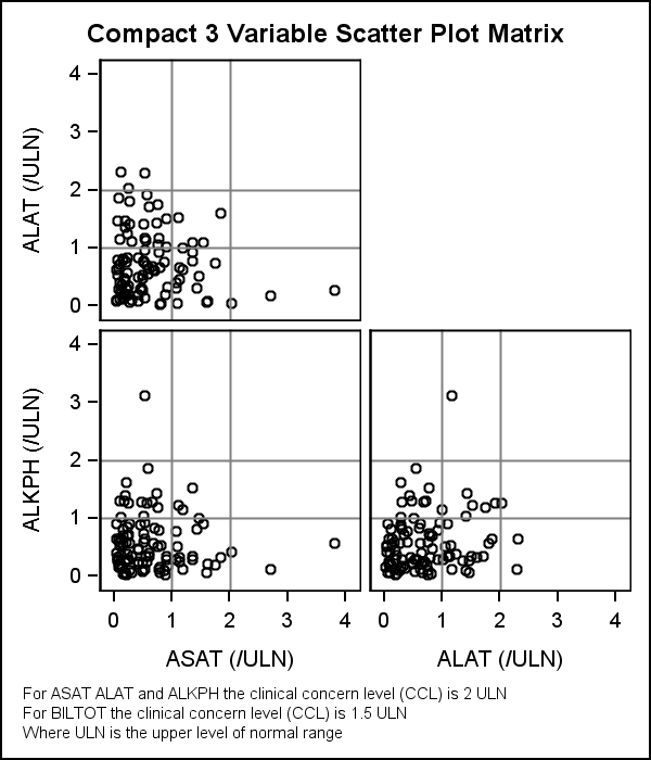
Macro invocation for 3-variable Compact Matrix:
%CompactMatrixMacro(data=safety, var1=asat, var2=alat, var3=alkph, title=Compact 3 Variable Scatter Plot Matrix, footnote=For ASAT ALAT and ALKPH the clinical concern level (CCL) is 2 ULN, footnote2=For BILTOT the clinical concern level (CCL) is 1.5 ULN, footnote3=Where ULN is the upper level of normal range, titlefontsize=9, footnotefontsize=6, axisvalueincr=1); |
Compact Matrix for 5 variables:
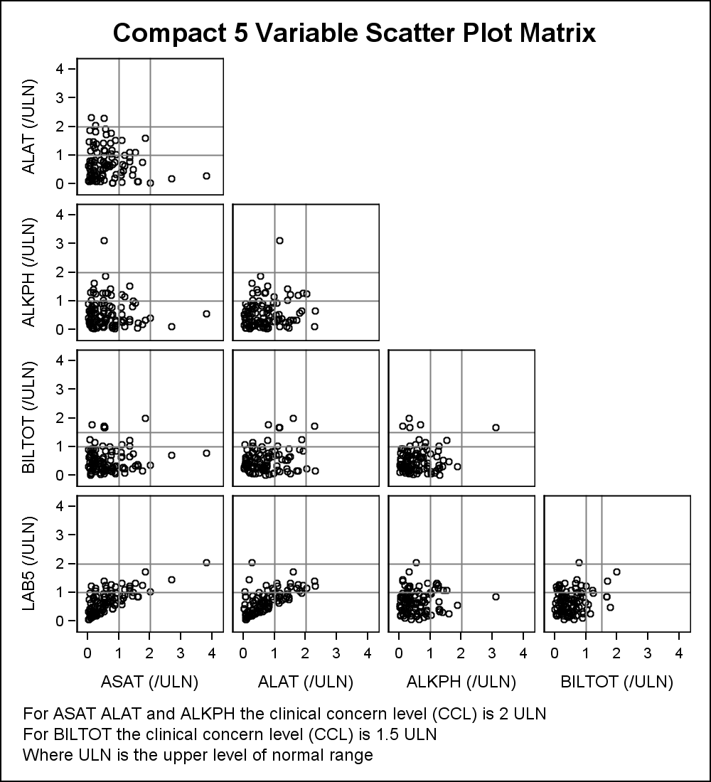
Macro invocation for 5-variable Compact Matrix:
%CompactMatrixMacro(data=safety, var1=asat, var2=alat, var3=alkph, var4=biltot, var5=lab5, title=Compact 5 Variable Scatter Plot Matrix, footnote=For ASAT ALAT and ALKPH the clinical concern level (CCL) is 2 ULN, footnote2=For BILTOT the clinical concern level (CCL) is 1.5 ULN, footnote3=Where ULN is the upper level of normal range, footnotefontsize=8, axisvalueincr=1); |
The CompactMatrixMacro has the following features:
- The macro accepts 3, 4 or 5 variables.
- You can provide the upper CCL levels for each variable.
- The lower CCL level is set to 1.0.
- You can set axis range (same for all variables).
- You can set two titles and 3 footnotes, each with its own text font size.
Caveat Emptor: The macro is for illustration purposes only, not bullet proof and not tested.
Macro program and invocation code is attached: CompactMatrixMacro_Code


6 Comments
Is it possible (or easy anyway) to modify this to include the histograms back in? I really like having them and the ability to control the axes, even if it's not any more compact than the original.
I would think you can do that. Here are the steps for the process:
1. Build the full N x N matrix.
2. Populate only the lower triangle with scatter plots.
3. Add Histograms to the diagonal elements.
4. Set external axes with the appropriate axis ranges.
5. Turn off the display of axis for the top row and right column.
6. Put a Layout Overlay around each histograms to decouple its axis with the common external axis.
How can I add a title above each of the individual graphs?
Note that I was able to use a "layout gridded" step to get what i needed.
layout lattice code that allows one to enter any # of variables (> 2):
layout lattice / columns=%eval(&numvars - 1) rows=%eval(&numvars - 1) rowgutter=5 columngutter=5
rowdatarange=union columndatarange=union;
* set common row options;
rowaxes;
%do k = 1 %to %eval(&numvars - 1);
rowaxis / tickvalueattrs=(size=7pt) labelattrs=(size=10pt) griddisplay=on
linearopts=(tickvaluesequence=(start=&axismin end=&axismax increment=&axisincr)
tickvaluepriority=true);
%end;
endrowaxes;
* set common column options;
columnaxes;
%do l = 1 %to %eval(&numvars - 1);
columnaxis / tickvalueattrs=(size=7pt) labelattrs=(size=10pt) griddisplay=on
linearopts=(tickvaluesequence=(start=&axismin end=&axismax increment=&axisincr)
tickvaluepriority=true);
%end;
endcolumnaxes;
%do n = 2 %to &numvars;
%do m = 1 %to %eval(&numvars - 1);
%if &m < &n %then %do;
* draw individual scatter plots;
layout overlay;
scatterplot y=&&var&n x=&&var&m / datalabel=&labelvar datalabelposition=center markerattrs=(size=0);
endlayout;
* add blank squares;
%if &n = %eval(&m + 1) %then %do o = 1 %to %eval(&numvars - &n);
layout overlay; entry ''; endlayout;
%end;
%end; %end; %end;
endlayout;
I have managed to expand to be a compact graph of 6 variables which is great.
However, my variables have quite different ranges of results so I would like to let each row have a different range of the y axis and each column to have a different range on the x axis. Then I don't want the values printed on the plots other than on the outside of the matrix. Any suggestions?
The other thing I am trying to do is put the estimated correlation for each panel somewhere on the corresponding plot. I thought I might be able to do it with annotate but can't see how to apply the annotated dataset to the template.