This resource is designed primarily for beginner to intermediate data scientists or analysts who are interested in identifying and applying machine learning algorithms to address the problems of their interest.
A typical question asked by a beginner, when facing a wide variety of machine learning algorithms, is “which algorithm should I use?” The answer to the question varies depending on many factors, including:
- The size, quality, and nature of data.
- The available computational time.
- The urgency of the task.
- What you want to do with the data.
Even an experienced data scientist cannot tell which algorithm will perform the best before trying different algorithms. We are not advocating a one-and-done approach, but we do hope to provide some guidance on which algorithms to try first depending on some clear factors.
Editor's note: This post was originally published in 2017. We are republishing it with an updated video tutorial on this topic. You can watch How to Choose a Machine Learning Algorithm below. Or keep reading to find a cheat sheet that helps you find the right algorithm for your project.
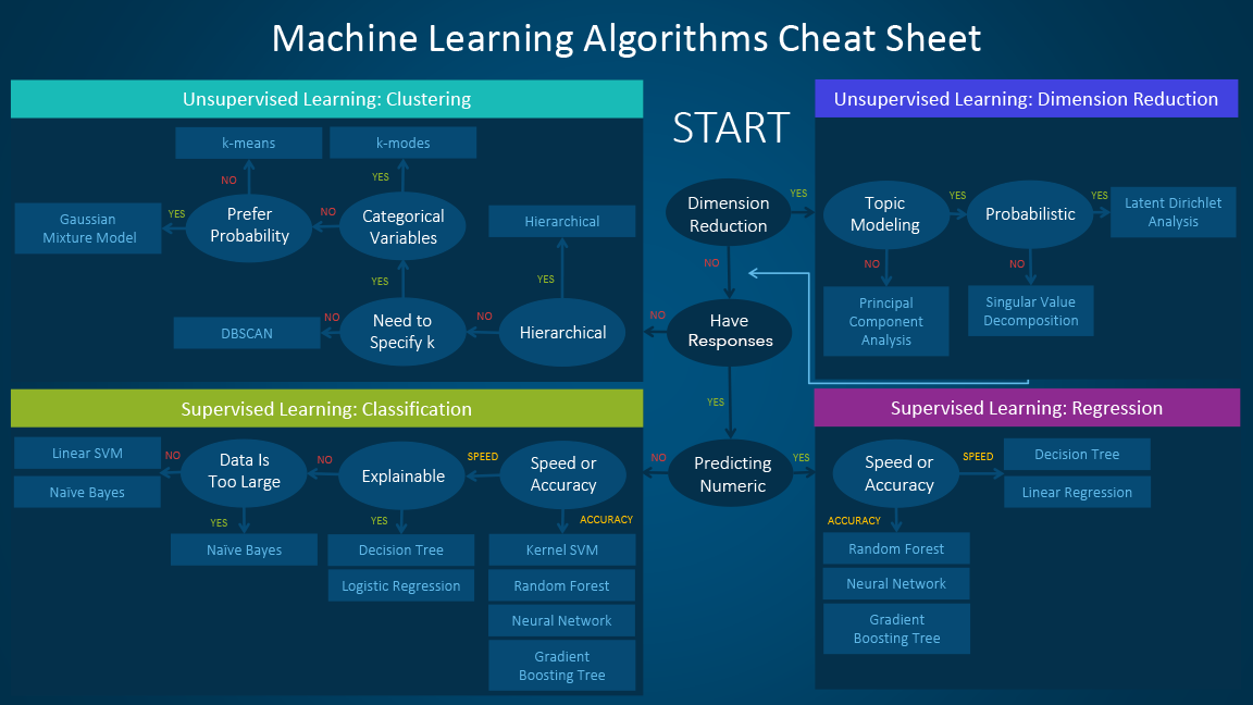
The machine learning algorithm cheat sheet
The machine learning algorithm cheat sheet helps you to choose from a variety of machine learning algorithms to find the appropriate algorithm for your specific problems. This article walks you through the process of how to use the sheet.
Since the cheat sheet is designed for beginner data scientists and analysts, we will make some simplified assumptions when talking about the algorithms.
The algorithms recommended here result from compiled feedback and tips from several data scientists and machine learning experts and developers. There are several issues on which we have not reached an agreement and for these issues, we try to highlight the commonality and reconcile the difference.
Additional algorithms will be added in later as our library grows to encompass a more complete set of available methods.
How to use the cheat sheet
Read the path and algorithm labels on the chart as "If <path label> then use <algorithm>." For example:
- If you want to perform dimension reduction then use principal component analysis.
- If you need a numeric prediction quickly, use decision trees or linear regression.
- If you need a hierarchical result, use hierarchical clustering.
Sometimes more than one branch will apply, and other times none of them will be a perfect match. It’s important to remember these paths are intended to be rule-of-thumb recommendations, so some of the recommendations are not exact. Several data scientists I talked with said that the only sure way to find the very best algorithm is to try all of them.
Types of machine learning algorithms
This section provides an overview of the most popular types of machine learning. If you’re familiar with these categories and want to move on to discussing specific algorithms, you can skip this section and go to “When to use specific algorithms” below.
Supervised learning
Supervised learning algorithms make predictions based on a set of examples. For example, historical sales can be used to estimate future prices. With supervised learning, you have an input variable that consists of labeled training data and a desired output variable. You use an algorithm to analyze the training data to learn the function that maps the input to the output. This inferred function maps new, unknown examples by generalizing from the training data to anticipate results in unseen situations.
- Classification: When the data are being used to predict a categorical variable, supervised learning is also called classification. This is the case when assigning a label or indicator, either dog or cat to an image. When there are only two labels, this is called binary classification. When there are more than two categories, the problems are called multi-class classification.
- Regression: When predicting continuous values, the problems become a regression problem.
- Forecasting: This is the process of making predictions about the future based on past and present data. It is most commonly used to analyze trends. A common example might be an estimation of the next year sales based on the sales of the current year and previous years.
Semi-supervised learning
The challenge with supervised learning is that labeling data can be expensive and time-consuming. If labels are limited, you can use unlabeled examples to enhance supervised learning. Because the machine is not fully supervised in this case, we say the machine is semi-supervised. With semi-supervised learning, you use unlabeled examples with a small amount of labeled data to improve the learning accuracy.
Unsupervised learning
When performing unsupervised learning, the machine is presented with totally unlabeled data. It is asked to discover the intrinsic patterns that underlie the data, such as a clustering structure, a low-dimensional manifold, or a sparse tree and graph.
- Clustering: Grouping a set of data examples so that examples in one group (or one cluster) are more similar (according to some criteria) than those in other groups. This is often used to segment the whole dataset into several groups. Analysis can be performed in each group to help users to find intrinsic patterns.
- Dimension reduction: Reducing the number of variables under consideration. In many applications, the raw data have very high dimensional features and some features are redundant or irrelevant to the task. Reducing the dimensionality helps to find the true, latent relationship.
Reinforcement learning
Reinforcement learning is another branch of machine learning which is mainly utilized for sequential decision-making problems. In this type of machine learning, unlike supervised and unsupervised learning, we do not need to have any data in advance; instead, the learning agent interacts with an environment and learns the optimal policy on the fly based on the feedback it receives from that environment. Specifically, in each time step, an agent observes the environment’s state, chooses an action, and observes the feedback it receives from the environment. The feedback from an agent’s action has many important components. One component is the resulting state of the environment after the agent has acted on it. Another component is the reward (or punishment) that the agent receives from performing that particular action in that particular state. The reward is carefully chosen to align with the objective for which we are training the agent. Using the state and reward, the agent updates its decision-making policy to optimize its long-term reward. With the recent advancements of deep learning, reinforcement learning gained significant attention since it demonstrated striking performances in a wide range of applications such as games, robotics, and control. To see reinforcement learning models such as Deep-Q and Fitted-Q networks in action, check out this article.
Considerations when choosing an algorithm
When choosing an algorithm, always take these aspects into account: accuracy, training time and ease of use. Many users put the accuracy first, while beginners tend to focus on algorithms they know best.
When presented with a dataset, the first thing to consider is how to obtain results, no matter what those results might look like. Beginners tend to choose algorithms that are easy to implement and can obtain results quickly. This works fine, as long as it is just the first step in the process. Once you obtain some results and become familiar with the data, you may spend more time using more sophisticated algorithms to strengthen your understanding of the data, hence further improving the results.
Even in this stage, the best algorithms might not be the methods that have achieved the highest reported accuracy, as an algorithm usually requires careful tuning and extensive training to obtain its best achievable performance.
When to use specific algorithms
Looking more closely at individual algorithms can help you understand what they provide and how they are used. These descriptions provide more details and give additional tips for when to use specific algorithms, in alignment with the cheat sheet.
Linear regression and Logistic regression
-
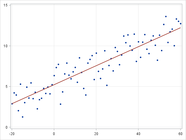
- Linear regression
-
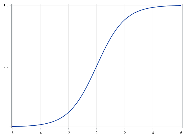
- Logistic regression
Linear regression is an approach for modeling the relationship between a continuous dependent variable \(y\) and one or more predictors \(X\). The relationship between \(y\) and \(X\) can be linearly modeled as \(y=\beta^TX+\epsilon\) Given the training examples \(\{x_i,y_i\}_{i=1}^N\), the parameter vector \(\beta\) can be learnt.
If the dependent variable is not continuous but categorical, linear regression can be transformed to logistic regression using a logit link function. Logistic regression is a simple, fast yet powerful classification algorithm. Here we discuss the binary case where the dependent variable \(y\) only takes binary values \(\{y_i\in(-1,1)\}_{i=1}^N\) (it which can be easily extended to multi-class classification problems).
In logistic regression we use a different hypothesis class to try to predict the probability that a given example belongs to the "1" class versus the probability that it belongs to the "-1" class. Specifically, we will try to learn a function of the form:\(p(y_i=1|x_i )=\sigma(\beta^T x_i )\) and \(p(y_i=-1|x_i )=1-\sigma(\beta^T x_i )\). Here \(\sigma(x)=\frac{1}{1+exp(-x)}\) is a sigmoid function. Given the training examples\(\{x_i,y_i\}_{i=1}^N\), the parameter vector \(\beta\) can be learnt by maximizing the log-likelihood of \(\beta\) given the data set.
-
- Group By Linear Regression
-
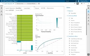
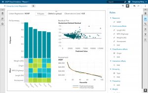
- Logistic Regression in SAS Visual Analytics
Linear SVM and kernel SVM
Kernel tricks are used to map a non-linearly separable functions into a higher dimension linearly separable function. A support vector machine (SVM) training algorithm finds the classifier represented by the normal vector \(w\) and bias \(b\) of the hyperplane. This hyperplane (boundary) separates different classes by as wide a margin as possible. The problem can be converted into a constrained optimization problem:
\begin{equation*}
\begin{aligned}
& \underset{w}{\text{minimize}}
& & ||w|| \\
& \text{subject to}
& & y_i(w^T X_i-b) \geq 1, \; i = 1, \ldots, n.
\end{aligned}
\end{equation*}
A support vector machine (SVM) training algorithm finds the classifier represented by the normal vector and bias of the hyperplane. This hyperplane (boundary) separates different classes by as wide a margin as possible. The problem can be converted into a constrained optimization problem:
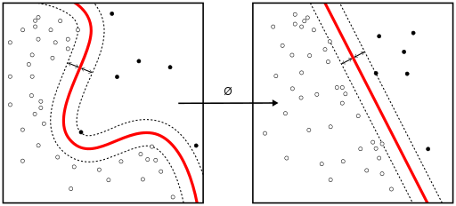
When the classes are not linearly separable, a kernel trick can be used to map a non-linearly separable space into a higher dimension linearly separable space.
When most dependent variables are numeric, logistic regression and SVM should be the first try for classification. These models are easy to implement, their parameters easy to tune, and the performances are also pretty good. So these models are appropriate for beginners.
Trees and ensemble trees
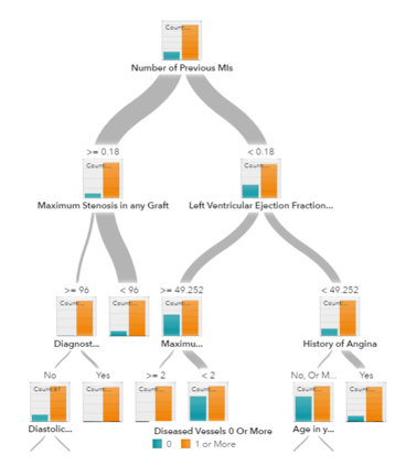
Decision trees, random forest and gradient boosting are all algorithms based on decision trees. There are many variants of decision trees, but they all do the same thing – subdivide the feature space into regions with mostly the same label. Decision trees are easy to understand and implement. However, they tend to over-fit data when we exhaust the branches and go very deep with the trees. Random Forrest and gradient boosting are two popular ways to use tree algorithms to achieve good accuracy as well as overcoming the over-fitting problem.
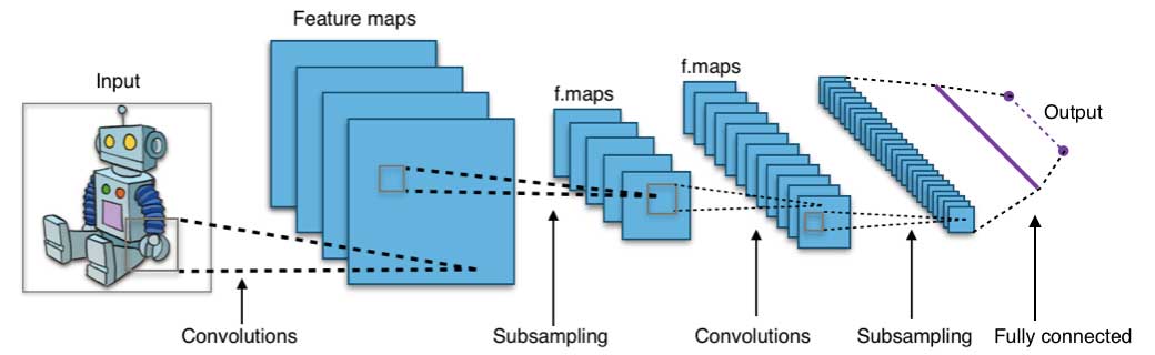
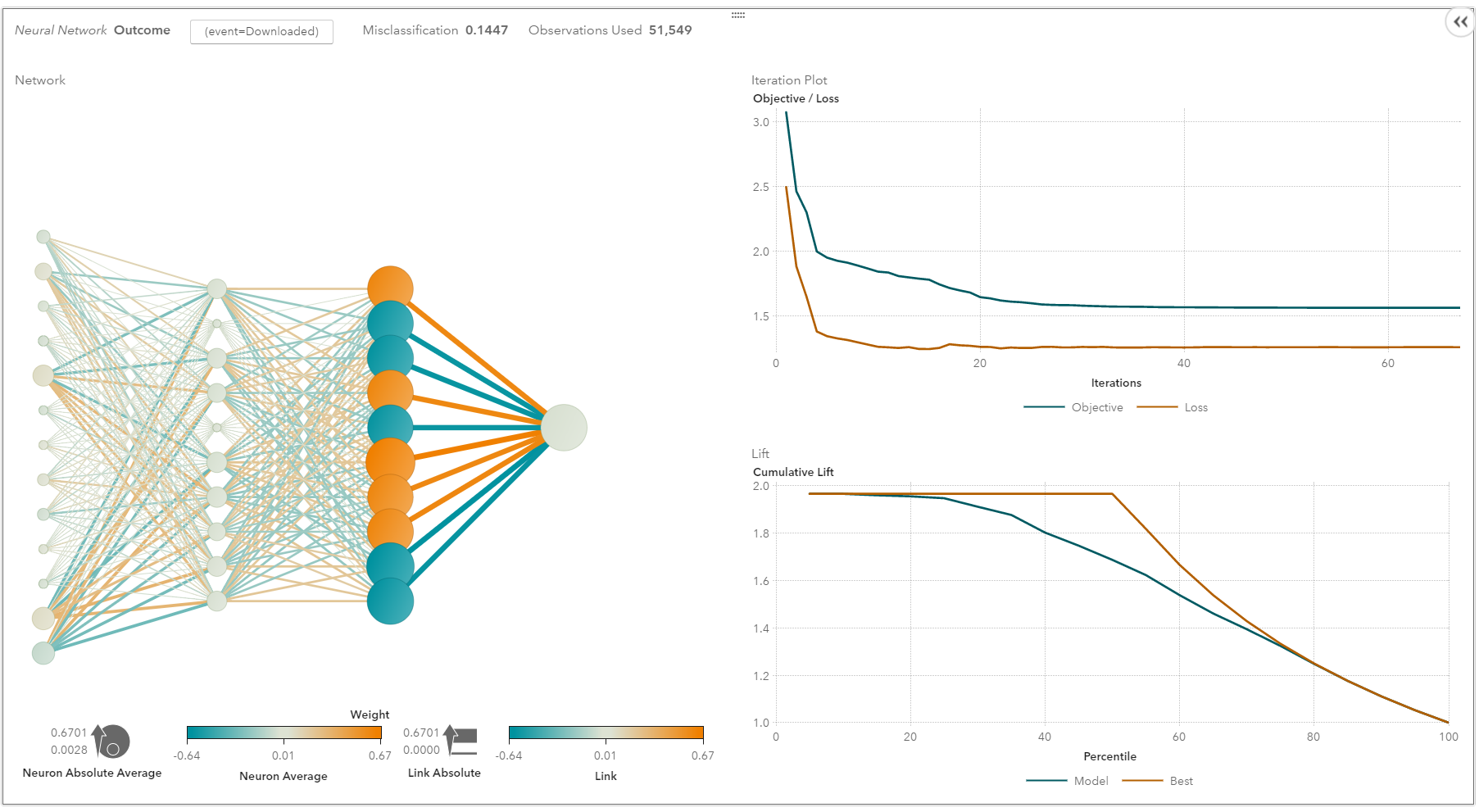
Neural networks and deep learning
Neural networks flourished in the mid-1980s due to their parallel and distributed processing ability. But research in this field was impeded by the ineffectiveness of the back-propagation training algorithm that is widely used to optimize the parameters of neural networks. Support vector machines (SVM) and other simpler models, which can be easily trained by solving convex optimization problems, gradually replaced neural networks in machine learning.
In recent years, new and improved training techniques such as unsupervised pre-training and layer-wise greedy training have led to a resurgence of interest in neural networks. Increasingly powerful computational capabilities, such as graphical processing unit (GPU) and massively parallel processing (MPP), have also spurred the revived adoption of neural networks. The resurgent research in neural networks has given rise to the invention of models with thousands of layers.
In other words, shallow neural networks have evolved into deep learning neural networks. Deep neural networks have been very successful for supervised learning. When used for speech and image recognition, deep learning performs as well as, or even better than, humans. Applied to unsupervised learning tasks, such as feature extraction, deep learning also extracts features from raw images or speech with much less human intervention.
A neural network consists of three parts: input layer, hidden layers and output layer. The training samples define the input and output layers. When the output layer is a categorical variable, then the neural network is a way to address classification problems. When the output layer is a continuous variable, then the network can be used to do regression. When the output layer is the same as the input layer, the network can be used to extract intrinsic features. The number of hidden layers defines the model complexity and modeling capacity.
Deep Learning: What it is and why it mattersk-means/k-modes, GMM (Gaussian mixture model) clustering
-
- K Means Clustering
-
- Gaussian Mixture Model
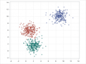
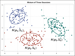
Kmeans/k-modes, GMM clustering aims to partition n observations into k clusters. K-means define hard assignment: the samples are to be and only to be associated to one cluster. GMM, however, defines a soft assignment for each sample. Each sample has a probability to be associated with each cluster. Both algorithms are simple and fast enough for clustering when the number of clusters k is given.
DBSCAN
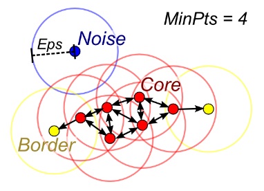
When the number of clusters k is not given, DBSCAN (density-based spatial clustering) can be used by connecting samples through density diffusion.
Hierarchical clustering
Hierarchical partitions can be visualized using a tree structure (a dendrogram). It does not need the number of clusters as an input and the partitions can be viewed at different levels of granularities (i.e., can refine/coarsen clusters) using different K.
PCA, SVD and LDA
We generally do not want to feed a large number of features directly into a machine learning algorithm since some features may be irrelevant or the “intrinsic” dimensionality may be smaller than the number of features. Principal component analysis (PCA), singular value decomposition (SVD), and latent Dirichlet allocation (LDA) all can be used to perform dimension reduction.
PCA is an unsupervised clustering method that maps the original data space into a lower-dimensional space while preserving as much information as possible. The PCA basically finds a subspace that most preserve the data variance, with the subspace defined by the dominant eigenvectors of the data’s covariance matrix.
The SVD is related to PCA in the sense that the SVD of the centered data matrix (features versus samples) provides the dominant left singular vectors that define the same subspace as found by PCA. However, SVD is a more versatile technique as it can also do things that PCA may not do. For example, the SVD of a user-versus-movie matrix is able to extract the user profiles and movie profiles that can be used in a recommendation system. In addition, SVD is also widely used as a topic modeling tool, known as latent semantic analysis, in natural language processing (NLP).
A related technique in NLP is latent Dirichlet allocation (LDA). LDA is a probabilistic topic model and it decomposes documents into topics in a similar way as a Gaussian mixture model (GMM) decomposes continuous data into Gaussian densities. Differently from the GMM, an LDA models discrete data (words in documents) and it constrains that the topics are a priori distributed according to a Dirichlet distribution.
Conclusions
This is the work flow which is easy to follow. The takeaway messages when trying to solve a new problem are:
- Define the problem. What problems do you want to solve?
- Start simple. Be familiar with the data and the baseline results.
- Then try something more complicated.
SAS Visual Data Mining and Machine Learning provides a good platform for beginners to learn machine learning and apply machine learning methods to their problems. Sign up for a free trial today!
WANT MORE GREAT INSIGHTS MONTHLY? | SUBSCRIBE TO THE SAS TECH REPORT


12 Comments
Thank you for the cheat-sheet, it provides a nice taxonomy for people to understand the relationship between algorithms. I will use it in my machine learning class to help students round out their world view.
Thank Daymond.
Let us know if you have any questions when teaching the students using the information.
This is a great cheat-sheet to understand and remember the relationship between the most usual machine learning algorithms. I have not seen something similar like this published online yet.
I think it could be nice to incorporate the "cost" variable, the principal’s reasons why each selection has been made and some examples of applications for each one. I know that this suggestion means a lot of work and scape from a cheat-sheet idea. Anyway, it could be a nice new project to be done, don’t you think so?
Congratulations for the work already done anyway!
Thanks, Hector. Incorporating the "cost" variable is a pretty wider area in machine learning. Actually it can be considered as a subfield of reinforcement learning -- based on the cost (reward), the agent determines the actions that he/she wants to take. I considered this problem for a while and haven't found a good example (or real user case) for it. If I have a time, I will write a blog specifically for the reinforcement learning.
An excellent blog. Thank you
Thank you.
Excellent summary but I think the target audience is a few steps beyond "beginner". I showed this to some folks just starting to study machine learning, and they were overwhelmed.
Great blog, thank you. I will use it when talking to non tech companies about starting doing ML and DL with their data sets.
Very helpful and concise, I was saddened to read that the author passed away in March 2019.
Pingback: Collaborative Filtering and Supervised Learning: A Tale of Two Methods - The SAS Data Science Blog
Pingback: See how composite AI benefits retailers, doctors and bankers - SAS Voices
Interesting post, thanks for sharing.