“Dear Cat, In a repeated measures drug study, I am unsure what to do with the baseline measurement. Since it is one of the time points in my study, I feel like I should use it as one of the dependent variable measurements. But I have seen analyses where baseline is treated as a predictor variable instead. Which one is correct? The model is a hierarchical linear model using PROC MIXED. Signed, Repeatedly Uncertain”
Dear Rep,
Put aside your baseline measurement woes, and grab a hot cocoa and some holiday frosted cookies. This will be worth the calories.
In repeated measures experiments, it is common to have some pre-treatment, or baseline, measurement of the dependent variable. This is useful for several reasons. First, you can make sure that your randomization scheme resulted in groups of patients who had similar responses, on average, to begin with. Second, if there is some difference between groups on the response, you can use the baseline measure as a covariate, interacting with the treatment (drug), to statistically account for those differences. Third (and most important), you can look at how your treatment changes the response for the patients compared to the baseline. This is easily done by computing a change from baseline as a dependent variable. When you do this, the tests of whether the response differs significantly from 0 are useful!
There are lots of other cool ways to assess whether the treatment was effective that I won’t go into here.
Let’s talk about two ways to handle baselines in your multilevel model:
- using baseline as a time point measurement
- using baseline as a covariate
By the way, repeated measures mixed model analysis is taught in the course Mixed Models Analyses Using SAS.
Scenario:
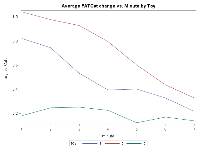
Suppose you were interested in the effect of catnip toys (two brands of catnip toy and a third placebo toy) on Friskiness Activation Test for Cats* score (FATCat). To help you identify the best brand, 72 cats are measured for baseline FATCat, and then randomly assigned to receive one of the three toys. FATCat is then measured each minute for the next 7 minutes (higher values of FATCat mean that the cat is having a bigger catnip high). There are eight repeated measurements of FATCat, including the baseline. Here’s a snapshot of the average response for each toy group:
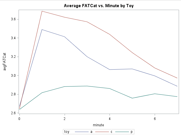
It appears that the baseline measurements are similar for the three groups of kitties. For the two active catnip toys (a and c), there appears to be a sharp increase in FATCat immediately after treatment, followed by a gradual return toward baseline. The placebo (p) shows a small bump in FATCat (wishful frisking?) but then hovers close to baseline for the duration of the follow-up measurements.
How to model this? What to do with that pesky baseline?
Pesky baseline: Notice the dogleg (pun not intended) from time 0 to the rest of the time points. Note that the analyst wants to treat time as a continuous variable.
Approach 1: Use baseline as a time point measurement and fit a piecewise linear mixed model. You’ll have essentially two different intercepts and a slope that starts after the treatment is given.
Approach 2: Use baseline as a covariate. You’ll have a simpler model with slightly fewer parameters and all effects are conditioned on the baseline measurement. This model might or might not use a deviation from baseline (Change-in-FATCat or FATCatdiff) as a dependent variable, depending on whether it is more important to interpret and predict the absolute level of FATCat, or the change in FATCat from baseline.
Click here to see how to do it in SAS PROC MIXED. For example:
By the way, if frisky kitties are not your thing, Littel, et al.’s book, SAS for Mixed Models, Chapter 16 has a different example. It’s a terrific book, and makes a nice stocking stuffer for your dearest analytically-minded friends.
You’ll recall that we are interested in FATCat measurements on 72 cats taken each minute for 7 minutes after administration of a catnip (or placebo) toy.
APPROACH #1 Using baseline as a time point measurement: Fitting a mean model with this dogleg pattern is a little tricky, but you can do it with a piece-wise fit. To accomplish this, you will need two intercepts: one for baseline, and one for after baseline. You will also need the slope to start after baseline since there should be no effect of toy on baseline (unless, of course, your cats can time travel).
Your random coefficients also need to reflect different intercepts for baseline and after baseline as well as the random slopes for minute. This complicates your model a bit and increases the number of covariance parameters being estimated. I’ll show you all of this below.
First, you will need to create variables to fit the piece-wise regression. Posttest is a binary variable to identify the post-treatment observations. Minutex is the time variable, offset to 0 for the post-treatment observations.
posttest=minute gt 0; if minute ne 0 then minutex = minute-1; else minutex = 0; |
The new variable posttest takes on a value of 0 if the measurement is minute 0 and 1 otherwise (there are no missing minutes, so this simple line of code works well). Minutex remains 0 for baseline, but shifts the post-treatment minutes back by 1 so that the first posttest minute = 0.
Here’s the PROC MIXED syntax for the piecewise linear fit:
proc mixed data=FATCat_8; class toy cat; model FATCat= posttest toy*posttest minutex toy*minutex /ddfm=kr solution outp=pred; random int posttest minutex / subject=cat(toy) type=un g; run; |
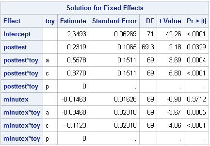
Fixed effects: The model statement has an implicit intercept, which will yield the mean of FATCat at baseline. The variable posttest provides the new intercept shift after treatment is administered for toy p (the reference level). The toy*posttest effect provides 2 parameters, the intercept deviations from toy p for toys a and c, all post-treatment. The effect minutex provides the slope for the post-treated minutes for toy p, and toy*minutex gives deviations from that slope for toys a and c. In total, seven fixed effect parameters are estimated:
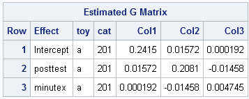
Random effects: The random intercept, posttest, and minutex effects allow for cat-to-cat variability in the two intercepts and the slope as described above. This results in a block-diagonal G matrix with 3x3 unstructured blocks for each cat, resulting in six estimated covariance parameters:
You can write estimate statements to get predictions for specific minute and toy combinations, and even get predictions for specific cats. Come to class if you want to learn those cool tricks.
Here’s a plot of the model-implied trajectories for the cats:
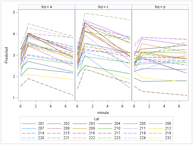
Can’t you just see those frisky kitties jumping about? These are the cat-specific predictions of FATCat, including baseline.
APPROACH #2 Using baseline as a covariate: Another way to look at this is as a deviation from baseline, and in some ways this is easier than the first approach I showed above. Look over the seven (post-treatment) average measurements of change from baseline for the three toys:
The dogleg is no longer apparent because the baseline is not part of the response (which, I’m sure, will make the cats happier). Instead, baseline is included in the model as a covariate. As before, the greatest change from baseline appears to be among the group who received active catnip brand c, followed by catnip brand a. The placebo group does not show much change from baseline. Now to fit the model!
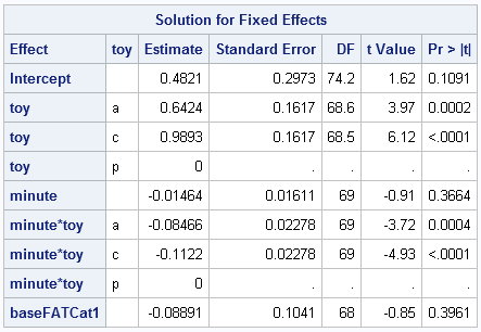
proc mixed data=FATCat_7; class toy cat; model FATCatdiff= toy minute toy*minute baseFATCat /ddfm=kr solution outp=pred; random int minute / subject=cat(toy) type=un g; run; |
The code is more straightforward because there is just an ANCOVA for the mean model, with random intercepts and slopes for the cats. In other words, a no-frills multilevel model.
There are still seven fixed effect parameters estimated:
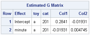
And with only two terms in the random statement, the blocks of G include have 3 estimated parameters (the intercept and slope variances, and the covariance between intercept and slopes):
The model implied trajectories for cats’ changes in FATCat are shown below:
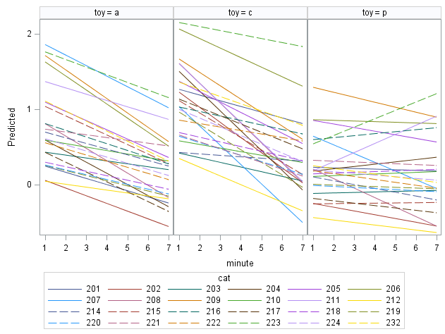
Not as frisky-looking of a plot, but just as easy to interpret. These are the predicted cat-specific changes in activity from baseline.
In addition to what I’m showing you here, Littel and colleagues have a handy table on page 717 that lists pros and cons of treating baseline as either a covariate or as a time point. See why it’s such a nice stocking stuffer? My mom already has her copy.
If you’re interested in learning more about models like this one, check out the course Mixed Models Analyses Using SAS.
Of course, you don’t have to use FATCatdiff as the DV here; you could simply use FATCat. The interpretation is different, but still quite useful. That holiday gift will have to be opened another day.
Maybe next year…


2 Comments
Hi Steve!
Good comment and thanks for the example code- I see that you favor a residual-side model for the repeated measures analysis instead of the random coefficient model approach -- that could be another good blog post right there!
There are differences (no pun intended) of opinion on whether to use the deviation from baseline as the dependent variable or not, and there can be value in either approach. As you correctly point out, using just FATCat as the DV gives you an interpretation of a "typical" baseline response. This is especially useful when the value of the DV is of interest, such as HDL or LDL cholestorol, for example, which has some absolute interpretation. I agree that in many studies, that is what you should use as the DV. So you're not the only one who prefers not to use differences and covariates.
It is also sometimes of value to see how much the treatment changed the DV relative to baseline, which gives a relative interpretation. In that case, it isn't the actual value of FATCat that matters, but the change in FATCat. If a very active cat is less active post-baseline, the value of FATCat might still be high-- but the deviation is negative, which tells you that the cat actually decreased compared to that cat's peculiar baseline activation level. Without baseline as a timepoint, you would miss this if you just modeled FATCat instead of the difference. This is also useful with, for example, measures that have some arbitrary scaling. Increases or decreases are more important than the actual value.
I agree that using baseline as a covariate with the difference as a DV makes the parameter estimates a little trickier to interpret, and for that reason, it isn't always the best choice. However, it does enable you to asses the change in the DV differs significantly by drug. And that can be useful to know. As I said in the post's last paragraph, it's a topic for another year!
Thanks for reading, and for leaving a comment!
Hi Cat,
Great presentation. Got to admit I have a problem with fitting the difference and the covariate. Consider that FATCATdiff = FATCAT - baseFATCAT. Now we have baseFATCAT on both sides of the model equation, in one case with a fixed coefficient of -1, and on the other side with a REML estimate of -0.08891. This leads to an almost inevitable misinterpretation of the effect of baseFATCAT on the actual measurement. Perhaps the following allows for an interpretation that is a little easier to follow:
proc mixed data=FATCat_7;
class toy cat minute;
model FATCat= toy minute toy*minute
baseFATCat /ddfm=kr solution outp=pred;
repeated minute / subject=cat(toy) type=un ;
run;
The linearity over time could be tested with an ESTIMATE statement. This analysis would give least squares means at each time point that are unbiased estimates, supposing that all animals had started at the same place (mean of baseFATCat). Thus, the effect of toy type is now independent of the starting value, which isn't really the case when you fit difference from baseline as a response, and include the baseline measure as a covariate.
Steve Denham