In a previous post, I discussed using discrete-event simulation to validate an optimization model and its underlying assumptions.  A similar approach can be used to validate queueing models as well.  And when it is found that the assumptions required for a queueing model are not a good fit for the real-world system under investigation, discrete-event simulation provides a flexible modeling alternative.  To demonstrate, let’s use a queueing theory model and discrete-event simulation to investigate a real-life system that has become quite popular in the NC Triangle area in recent years:  the Food Truck Rodeo.

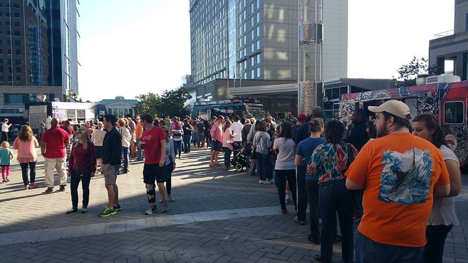
Four times a year, downtown Raleigh hosts a Food Truck Rodeo that includes a half mile of food trucks spread out over eleven city blocks.  Over 50 trucks from across NC participate with names like Wandering Moose, Stuft, and Bam Pow Chow, serving everything from Korean BBQ to cupcakes.  A local food truck called Pho Nomenal Dumpling was even named ‘Best Food Truck in America’ after participating in the Food Network’s Great Food Truck Race.

The Queueing Model

Let’s suppose that we are interested in attending the next food truck rodeo (where Pho Nomenal Dumpling will be participating) and we want to estimate how long we will have to wait in line at any given truck.  In the formulation of our queueing theory model, we can consider the food trucks to form a network of nodes.  Customers may arrive from outside the network to any node (i.e., truck) and may depart the network from any node.    Customers may return to nodes previously visited, or skip some nodes entirely.  The other assumptions for our queueing model are as follows:

1. There are $K$ trucks.
2. Customers arrive from outside the network to truck $i$ as a Poisson process with an average rate $\gamma_i$.
3. All servers at truck $i$ work according to an exponential distribution with average rate $\mu_i$.  All workers on a truck represent one service unit, rather than parallel servers.
4. When a customer completes service at truck $i$, he or she goes to truck $j$ next with probability $r_{ij}$, independent of the system state.  With probability $r_{i0}$ , a customer leaves the network at node $i$  upon completion of service (after receiving his or her food).
5. There is no limit on queue capacity at any truck.
6. There is a first-come-first-serve queueing discipline.

Queueing systems with these properties are called open (i.e., arrivals and departures from outside the network exist) Jackson networks. They have closed-form solutions for the expected waiting time in queue.  To compute the waiting time, we first compute the total arrival rate $\lambda_i$  into truck $i$ and then compute the utilization factor $\rho_i$ for the truck.

Now $\lambda_i$ has two components: the external arrival rate $\gamma_i$  into node $i$ and the probability-weighted sum of arrival rates from all other trucks $j$.  In summary, $\lambda_i = \gamma_i + \sum_{j=1}^{K} r_{ji} \lambda_{j}$.

The utilization factor $\rho_i$  is the ratio of the total arrival rate to the mean service time: $\rho_i=\frac{\lambda_i}{\mu_i}$.  It is a measure of the average use of the resource (in our case, a truck).  If $\rho_i \geq 1$, then the queue grows infinitely long, and so thus the average waiting time.  But if $\rho_i \lt 1$, then the expected waiting time $W_i$ at node $i$ is $W_i = \frac{\rho_i}{1-\rho_i}\frac{1}{\mu_i}$.

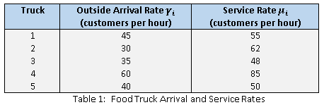
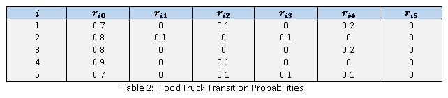
For this example, assume there are $K=5$  trucks participating in our food truck rodeo.  Table 1 below shows the mean arrival rate to each truck from outside the network, as well as the mean service rates.  Table 2 gives the probability $r_{ij}$ that a customer who has completed service and received his or her food at truck $i$ will go to truck $j$ next and get something else to eat.  We will assume truck 4 is the popular Pho Nomenal Dumpling truck.

Solving five equations in five unknowns for $\lambda_i, i=1,2,...,5$, we can compute the total mean flow rate $\lambda_i$ for each truck and then we can compute the utilization factor $\rho_i$ for each truck.  Table 3 shows these results, along with the expected waiting time (queueing time) at each truck.

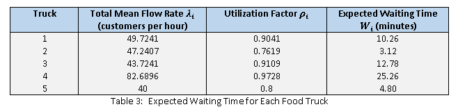
The expected waiting time that we computed for each truck in Table 3 using the Jackson Network model is the expected waiting time when the system is in steady-state.  But suppose we want to model the time spent waiting in line at each truck during a four-hour window around dinner time. Then, we are interested in a transient state.  In general, analytical solutions for transient queueing systems are impractically difficult to obtain.  How different is the steady state from this transient state?

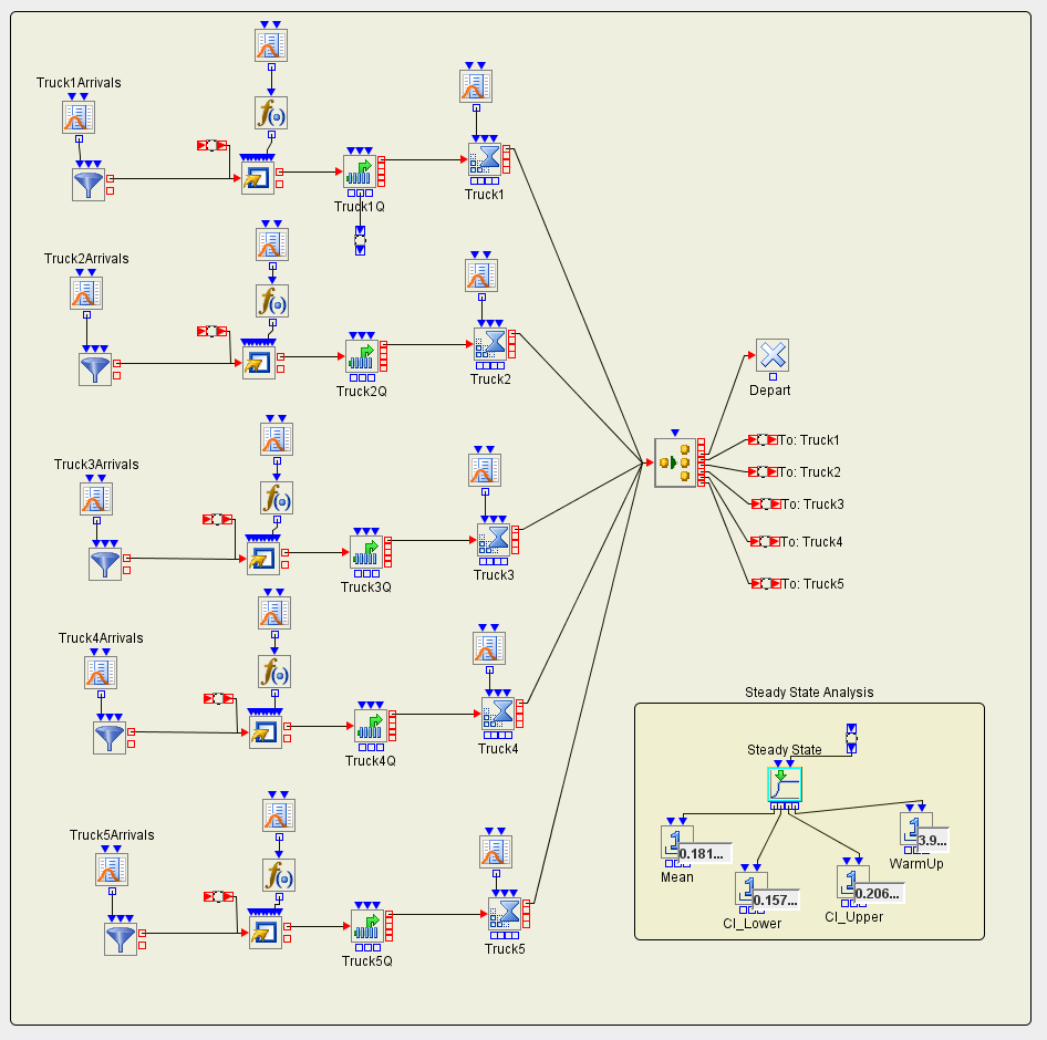
The Simulation Model

To answer that question, I built a discrete-event simulation model of our food truck rodeo system in SAS Simulation Studio 14.1  (shown below) and ran the model two ways.  First, I ran the simulation to steady state. Then, I ran the model for the more realistic simulated time of four hours (or approximately four hours since the model will continue to run until all customers that are still in the system at the end of four hours are served).

SAS Simulation Studio has a Steady State block to estimate the expected waiting time at each truck in steady-state operation.  Table 4 below shows the results of that simulation experiment.  As we should expect, the theoretical expected waiting times and those simulated using a sample agree almost exactly. The SAS Simulation Studio Steady State block provides a further measurement: an estimate of the time to reach steady-state operation.  Truck 4, the one with the longest waiting times, and thus the one whose performance is most important to estimate accurately, takes an alarmingly long time to reach steady-state.

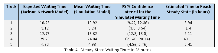
Food trucks typically operate for short time windows around lunch or dinner.  It is not likely that any food truck would remain open for the period of time required to reach steady-state operation (and certainly not 49 hours). So I then ran 100 independent replications of the simulation model, each with a run length of four hours (to represent a window around dinner time) and recorded the average waiting time across all replications for each truck. The results of this simulation experiment are shown in Table 5.

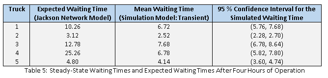
Table 5 demonstrates that the steady-state results do not reflect the behavior we observe if we run the system for four hours. I am pretty certain that the owners of the Pho Nomenal truck would not appreciate an overestimation of their expected waiting times by almost 19 minutes.

Before you get too excited about the relatively small amount of time you will have to wait to sample one of Pho Nomenal's dumplings, please note that all arrival rates and service rates in my food truck system are fictional.  To my colleague Leo Lopes, who suggested that I write this blog post, I now challenge you to hang out at the next food truck rodeo and collect actual arrival and service rates so we can all carefully plan out which food trucks to visit at the next rodeo.

Easy modeling of transient behavior is only one of the ways that SAS Simulation Studio enhances the analytics of queueing networks. The following simple (and realistic) changes to our food truck rodeo example also violate the assumptions underlying the Jackson Network model:

1. Suppose someone is waiting in line and sees someone else walk by with something yummy from another truck. The person decides to jump out of line and join the line for the other truck.
2. Suppose someone at a particular truck places an exceptionally large order. Naturally, the food truck workers are going to assist other customers in line behind that customer if they are able to do so.
3. Suppose a concert lets out and there is a rush of people to the food truck rodeo.

In future blog posts we will enhance our model to handle these conditions.