The primary objective of many discrete-event simulation projects is system investigation.  Output data from the simulation model are used to better understand the operation of the system (whether that system is real or theoretical), as well as to conduct various "what-if"-type analyses.   However, I recently worked on another model where the goal was to use simulation for validation, specifically, to validate the solution of an optimization model.  When constructing an optimization model, it is necessary to make certain simplifying assumptions, especially when there are various sources of randomness inherent in the process being modeled.  A common approach involves optimizing to some nominal value, like a mean, and then hoping for the best.  In order to validate an optimization model and its underlying assumptions, a simulation model of the process can be built that uses the optimal solution as an input and simulates the process under investigation as it evolves over time.  Essentially, the simulation model can be used to determine how the optimal solution holds up when randomness and perhaps other logical complexities (which the optimization model may have ignored or modeled only approximately) are introduced.

This simulation for validation technique was recently used for a major European utility company (which I will refer to as “SRG” for confidentiality reasons).   Here, I will give an overview of the project; the full paper can be found here.

Background

SRG provides on-site services to customers who call in for help when their furnace, water heater, or other gas-powered appliance needs repair or maintenance.  SRG receives approximately 10 million calls from its customers each year, and there are more than 10 types of calls, ranging from emergency breakdowns to annual maintenance.  Each call type is given a target service level that measures how it is served.  The service level is defined by two parameters: a time window and a percentage.  For example, if a customer calls in because his water heater has broken down and the call is made before 1 p.m., SRG must dispatch a service engineer to visit the customer the same day 90% of the time.  Here, the time window is “same day,” and the percentage is 90%.

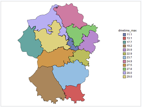
SRG employs several thousand service engineers, and its territory is organized in a hierarchical structure. Figure 1 shows one particular subregion that contains 14 work areas.  The legend gives, for each work area, the maximum drive time (in minutes) between any two postal sectors in that work area.

In recent years, SRG has noticed that its engineers spend a significant amount of time serving customers outside their designated work areas either because there simply are not enough engineers to handle all customer calls or because there is a mismatch between the skills of the engineers and the skills required to complete the customer calls.  The increased travel time not only reduces engineers’ availability to serve calls in their own areas but also increases overtime and subcontractor hours, which can be quite costly.

The primary goal of the project for SRG is to find a better configuration of its work areas in order to minimize the total travel time of its service engineers.  The secondary goal is to minimize the costs of overtime and subcontractors.  My colleague Jinxin Yi in the Advanced Analytics and Optimization Services team (formerly called the OR Center of Excellence) used SAS/OR to find the optimal configuration of work areas, a process that required three steps.

The Optimization Model

The first step in finding the optimal territory configuration is to generate potential work areas, and the second step is to evaluate those potential work areas based on how customer calls can be served by engineers.  The calls from customers in each work area can be thought of as “demand” and the work hours of service engineers in the area as “supply”.  A linear programming model finds the best way to match demand with supply in order to minimize the aggregated shortage of engineer hours.  For example, the aggregated shortage for the work areas in Figure 1 is approximately 38 hours on a daily basis.

The third step is to then select the optimal subset of potential work areas that cover SRG’s entire territory with the least amount of shortage.  A mixed integer linear programming model is developed for this purpose.  Figure 2 shows the new and optimal design of the work areas for the subregion shown in Figure 1.  The shortage in the new design is 9.7 hours, which is significantly less than that in the current work area design, with similar improvements for other parts of SRG’s service territory.

After reviewing this optimal work area configuration, SRG expressed some concern about how the solution would actually hold up in practice. Both the actual engineer drive times and the random arrival pattern of customer calls are extremely difficult to capture in the optimization model, and as a result, simplifying assumptions have to be made.  SRG’s main concerns were:

1. Would engineer drive times really be reduced with the optimal configuration? and
2. Would the desired percentage of calls of each type be served within the designated time window?

The best way to answer these questions is to build a discrete-event simulation model to validate the optimally configured work areas.

The Discrete-Event Simulation Model

SAS Simulation Studio 13.2 is used to simulate a random arrival pattern of customer service calls and the assignment of those calls to a service engineer over a six-month period.  The figure below shows a high-level view of the model in SAS Simulation Studio.  Each yellow square in the model is a compound block that can be opened to display the SAS Simulation Studio logic contained within.

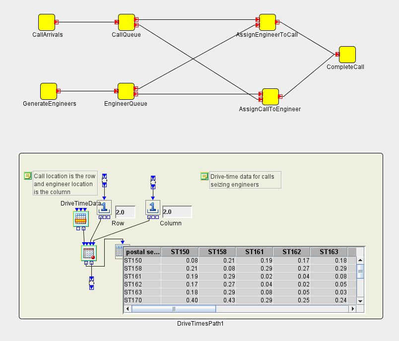
The inputs to the simulation model are in the form of SAS data sets and include drive-time data and the engineer data for an optimally configured work area.  In the bottom part of the model, the Dataset Holder block is used to hold the drive-time data set in memory so that it can be queried for each call.  The entities (or objects flowing through the model) represent customer calls and service engineers.  The customer call entities have attributes, or properties, that include call type, arrival time, and priority.  The engineer entities are generated at the start of the simulation for a specific work area, and their attributes (read in from a SAS data set) include starting location, hours worked, and skill set.  When a call entity is generated, it is sent to a queue where calls are prioritized according to the call type, arrival time, and desired time window.  The model then attempts to find an available engineer entity with the skill set required by the incoming call entity.  If no such engineer entity is available, then the call entity waits.  When a call entity is matched to an available engineer entity, a drive-time delay is computed based on the current locations of the call and the engineer, and a service-time delay is then determined based on the type of call.

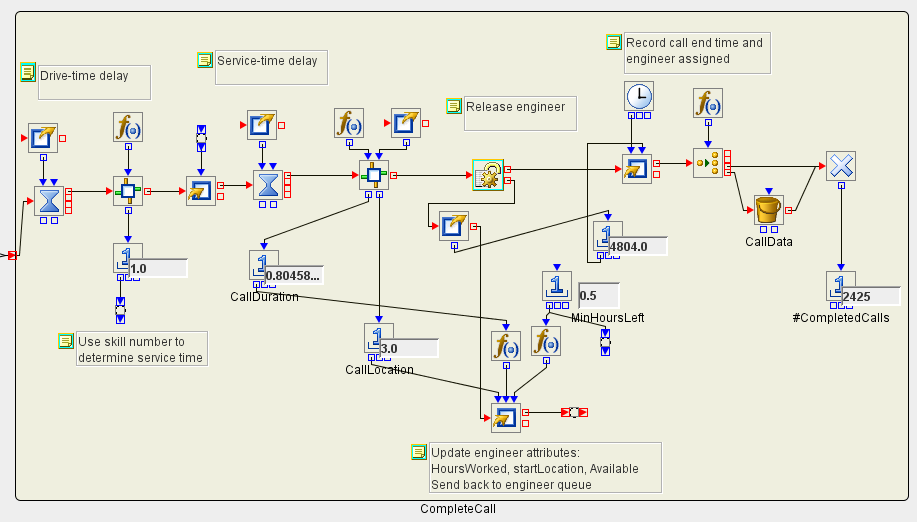
After the drive-time and service-time delays elapse, the call completion time is recorded, and all call attribute data (including engineer assigned, drive time, service time, and call completion time) are written to a SAS data set.  The figure below shows the expanded CompleteCall compound block in the SAS Simulation Studio model where this logic is executed.

When this simulation finished running, the recorded call data were analyzed.  For each work area simulated, 100% of the calls of each type fell within the desired call-completion time window.  The output data were also used to estimate the travel time of engineers, which indicated average drive-time reductions of up to 13%.

These results helped convince SRG that although additional factors not incorporated in the optimization model might affect the results, implementation of the proposed optimal work area configuration is expected to provide significant benefits.  Reducing the drive time between calls is expected to increase the number of calls that can be completed, with resulting improvement in meeting service levels and customer satisfaction.  Additional expected benefits include the ability to meet call demand with less use of overtime and subcontractors, which would reduce costs.

From the perspective of the SAS/OR development team, this project is the perfect example of how different OR techniques (here, optimization and simulation) can be used together in practice to not only solve a complex problem but to do so in a way that assures customer confidence in the validity of the solution.