A previous article discussed the mathematical properties of the singular value decomposition (SVD) and showed how to use the SVD subroutine in SAS/IML software. This article uses the SVD to construct a low-rank approximation to an image. Applications include image compression and denoising an image.

Construct a grayscale image

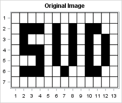
The value of each pixel in a grayscale image can be stored in a matrix where each element of the matrix is a value between 0 (off) and 1 (full intensity). I want to create a small example that is easy to view, so I'll create a small matrix that contains information for a low-resolution image of the capital letters "SVD." Each letter will be five pixels high and three pixels wide, arranges in a 7 x 13 array of 0/1 values. The following SAS/IML program creates the array and displays a heat map of the data:

ods graphics / width=390px height=210px;
proc iml;
SVD = {0 0 0 0 0 0 0 0 0 0 0 0 0,
       0 1 1 1 0 1 0 1 0 1 1 0 0,
       0 1 0 0 0 1 0 1 0 1 0 1 0,
       0 1 1 1 0 1 0 1 0 1 0 1 0,
       0 0 0 1 0 1 0 1 0 1 0 1 0,
       0 1 1 1 0 0 1 0 0 1 1 0 0,
       0 0 0 0 0 0 0 0 0 0 0 0 0 };
A = SVD;
/* ColorRamp:  White    Gray1    Gray2    Gray3    Black   */
ramp =        {CXFFFFFF CXF0F0F0 CXBDBDBD CX636363 CX000000};
call heatmapcont(A) colorramp=ramp showlegend=0 title="Original Image" range={0,1};

A low-rank approximation to an image

Because the data matrix contains only five non-zero rows, the rank of the A matrix cannot be more than 5. The following statements compute the SVD of the data matrix and create a plot of the singular values. The plot of the singular values is similar to the scree plot in principal component analysis, and you can use the plot to help choose the number of components to retain when approximating the data.

call svd(U, D, V, A);  /* A = U*diag(D)*V` */
title "Singular Values";
call series(1:nrow(D), D) grid={x y} xvalues=1:nrow(D) label={"Component" "Singular Value"};

For this example, it looks like retaining three or five components would be good choices for approximating the data. To see how low-rank approximations work, let's generate and view the rank-1, rank-2, and rank-3 approximations:

keep = 1:3;          /* use keep=1:5 to see all approximations */
do i = 1 to ncol(keep);
   idx = 1:keep[i];                           /* components to keep */
   Ak = U[ ,idx] * diag(D[idx]) * V[ ,idx]`;  /* rank k approximation */
   Ak = (Ak - min(Ak)) / range(Ak);           /* for plotting, stdize into [0,1] */
   s = "Rank = " + char(keep[i],1);
   call heatmapcont(Ak) colorramp=ramp showlegend=0 title=s range={0, 1};
end;

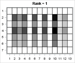
The rank-1 approximation does a good job of determining the columns and do not contain that contain the letters. The approximation also picks out two rows that contain the horizontal strokes of the capital "S."

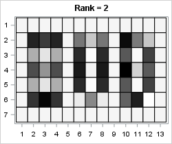
The rank-2 approximation refines the image and adds additional details. You can begin to make out the letters "SVD." In particular, all three horizontal strokes for the "S" are visible and you can begin to see the hole in the capital "D."

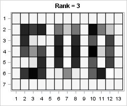
The rank-3 approximation contains enough details that someone unfamiliar with the message can read it. The "S" is reconstructed almost perfectly and the space inside the "V" and "D" is almost empty. Even though this data is five-dimensional, this three-dimensional approximation is very good.

Not only is a low-rank approximation easier to work with than the original five-dimensional data, but a low-rank approximation represents a compression of the data. The original image contains 7 x 13 = 91 values. For the rank-3 approximation, three columns of the U matrix contain 33 numbers and three columns of V^T contain 15 numbers. So the total number of values required to represent the rank-3 approximation is only 48, which is almost half the number of values as for the original image.

Denoising an image

You can use the singular value decomposition and low-rank approximations to try to eliminate random noise that has corrupted an image. Every TV detective series has shown an episode in which the police obtain a blurry image of a suspect's face or license plate. The detective asks the computer technician if she can enhance the image. With the push of a button, the blurry image is replaced by a crystal clear image that enables the police to identify and apprehend the criminal.

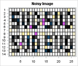
The image reconstruction algorithms used in modern law enforcement are more sophisticated than the SVD. Nevertheless, the SVD can do a reasonable job of removing small random noise from an image, thereby making certain features easier to see. The SVD has to have enough data to work with, so the following statements duplicate the "SVD" image four times before adding random Gaussian noise to the data. The noise has a standard deviation equal to 25% of the range of the data. The noisy data is displayed as a heat map on the range [-0.25, 1.25] by using a color ramp that includes yellow for negative values and blue for values greater than 1.

call randseed(12345);
A = (SVD // SVD) || (SVD // SVD);                     /* duplicate the image */
A = A + randfun( dimension(A), "Normal", 0, 0.25);    /* add Gaussian noise */
/*       Yellow   White    Gray1    Gray2    Gray3    Black    Blue    */
ramp2 = {CXFFEDA0 CXFFFFFF CXF0F0F0 CXBDBDBD CX636363 CX000000 CX3182BD};
call heatmapcont(A) colorramp=ramp2 showlegend=0 title="Noisy Image" range={-0.5, 1.5};

I think most police officers would be able to read this message in spite of the added noise, but let's see if the SVD can clean it up. The following statements compute the SVD and create a plot of the singular values:

call svd(U, D, V, A);  /* A = U*diag(D)*V` */
call series(1:nrow(D), D) grid={x y} xvalues=1:nrow(D) label={"Component" "Singular Value"};

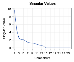
There are 14 non-zero singular values. In theory, the main signal is contained in the components that correspond to the largest singular values whereas the noise is captured by the components for the smallest singular values. For these data, the plot of the singular values suggests that three or five (or nine) components might capture the main signal while ignoring the noise. The following statements create and display the rank-3 and rank-5 approximations. Only the rank-5 approximation is shown.

keep = {3 5};        /* which components to examine? */
do i = 1 to ncol(keep);
   idx = 1:keep[i];
   Ak = U[ ,idx] * diag(D[idx]) * V[ ,idx]`;
   Ak = (Ak - min(Ak)) / range(Ak); /* for plotting, standardize into [0,1] */
   s = "Rank = " + char(keep[i],2);
   call heatmapcont(Ak) colorramp=ramp showlegend=0 title=s range={0, 1};
end;

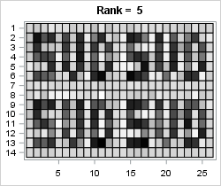
The denoised low-rank image is not as clear as Hollywood depicts, but it is quite readable. It is certainly good enough to identify a potential suspect. I can hear the detective mutter, "Book 'em, Danno! Murder One."

Summary and further reading

In summary, the singular value decomposition (SVD) enables you to approximate a data matrix by using a low-rank approximation. This article uses a small example for which the full data matrix is rank-5. A plot of the singular values can help you choose the number of components to retain. For this example, a rank-3 approximation represents the essential features of the data matrix.

For similar analyses and examples that use the singular value decomposition, see

• Austin, David (Aug 2009) "We Recommend a Singular Value Decomposition" (Mathematical)
• White, John Myles (Dec 2009) "Image Compression with the SVD in R"
• West Coast DSP (2015) "The Singular Value Decomposition and Image Processing" (MATLAB)
• For a longer and more detailed exposition, see the Master's Thesis of Workalemahu, Tsegaselassie (2008) "Singular Value Decomposition in Image Noise Filtering and Reconstruction", Georgia State University.

In SAS software, the SVD is heavily used in the SAS Text Miner product. For an overview of how a company can use text mining to analyze customer support issues, see Sanders and DeVault (2004) "Using SAS at SAS: The Mining of SAS Technical Support."