Students in introductory statistics courses often use summary statistics (such as sample size, mean, and standard deviation) to test hypotheses and to compute confidence intervals. Did you know that you can provide summary statistics (rather than raw data) to PROC TTEST in SAS and obtain hypothesis tests and confidence intervals? This article shows how to create a data set that contains summary statistics and how to call PROC TTEST to compute a two-sample or one-sample t test for the mean.
Did you know you that PROC TTEST in #SAS can analyze summary statistics? Click To TweetRun a two-sample t test for difference of means from summarized statistics
The documentation for PROC TTEST includes an example that shows how to compute a two-sample t test for the difference between the means of two groups. Rather than repeat the documentation example, let's compare the mean heights of 19 students based on gender. The data are contained in the Sashelp.Class data set.
To use PROC TTEST on summary statistics, the statistics must be in a SAS data set that contains a character variable named _STAT_ with values 'N', 'MEAN', and 'STD'. Because we are interested in a two-sample test, the data must also contain a grouping variable. The following SAS statements sort the data by the grouping variable, call PROC MEANS to write the summary statistics to a data set, and print a subset of the statistics:
proc sort data=sashelp.class out=class; by sex; /* sort by group variable */ run; proc means data=class noprint; /* compute summary statistics by group */ by sex; /* group variable */ var height; /* analysis variable */ output out=SummaryStats; /* write statistics to data set */ run; proc print data=SummaryStats label noobs; where _STAT_ in ("N", "MEAN", "STD"); var Sex _STAT_ Height; run; |
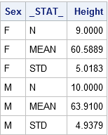
The table shows the structure of the SummaryStats data set for two-sample tests. The two samples are defined by the levels of the Sex variable ('F' for females and 'M' for males). The _STAT_ variable specifies the name of the statistics that are used in standard formulas for computing confidence intervals and hypothesis tests. The Height column shows the value of the statistics for each group.
You can use a data set like this one to conduct a two-sample t test of independent means. In a textbook, the problem is usually accompanied by a little story, like this:
The heights of sixth-grade students are normally distributed. Random samples of n1=9 females and n2=10 males are selected. The mean height of the female sample is m1=60.5889 with a standard deviation of s1=5.0183. The mean height of the male sample is m2=63.9100 with a standard deviation of s2=4.9379. Is there evidence that the mean height of sixth-grade students depends on gender?
The story suggests running a two-tailed test of the null hypothesis μ1 = μ2 against the alternative hypothesis that μ1 ≠ μ2. You do not have to do anything special to get PROC TTEST to use the summary statistics: if the procedure sees that the input data set contains a special variable named _STAT_ and the special values 'N', 'MEAN', and 'STD', then the procedure assumes that the data set contains summarized statistics. The following statements compare the mean heights of males and females for these students:
proc ttest data=SummaryStats order=data alpha=0.05 test=diff sides=2; /* two-sided test of diff between group means */ class sex; var height; run; |
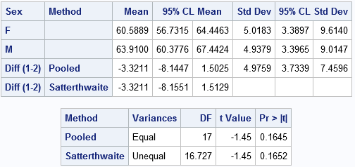
Notice that the output includes 95% confidence intervals for the group means, an estimate for the difference in means (-3.3211), and a confidence interval for the difference. You also get confidence intervals for the standard deviations.
In the second table, the "Pooled" row gives the t test under the assumption that the variances of the two groups are approximately equal, which seems to be true for these data. The value of the t statistic is t = -1.45 with a two-sided p-value of 0.1645. With this small sample, we fail to reject the null hypothesis at the 0.05 significance level. (For unequal group variances, use the "Satterthwaite" row.)
The syntax for the PROC TTEST statement enables you change the significance level and the type of hypothesis test. For example, to run a one-sided test for the alternative hypothesis μ1 < μ2 at the 0.10 significance level, you can use:
proc ttest ... alpha=0.10 test=diff sides=L; /* Left-tailed test */ |
Run a one-sample t test of the mean from summarized statistics
In the previous section, PROC MEANS generated the summary statistics. However, you can also create the summary statistics manually, which is useful when you do not have access to the original data. As before, the key requirements are a variable named _STAT_ that has values 'N', 'MEAN', and 'STD'.
For example, a Penn State online statistics course states the following problem:
A research study measured the pulse rates of 57 college men and found
a mean pulse rate of 70.4211 beats per minute with a standard deviation
of 9.9480 beats per minute. Researchers want to know if the mean pulse
rate for all college men is different from the current standard of 72
beats per minute.
The following SAS DATA step writes the summary statistics to a data set, then calls PROC TTEST to run a one-sample test of the null hypothesis μ = 72 against a two-sided alternative hypothesis:
data SummaryStats; infile datalines dsd truncover; input _STAT_:$8. X; datalines; N, 57 MEAN, 70.4211 STD, 9.9480 ; proc ttest data=SummaryStats alpha=0.05 H0=72 sides=2; /* H0: mu=72 vs two-sided alternative */ var X; run; |
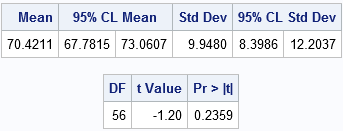
The results show that a 95% confidence interval for the mean contains the value 72. The value of the t statistic is t = -1.20, which corresponds to a p-value of 0.2359. Consequently, the data fails to reject the null hypothesis at the 0.05 significance level. These pulse rates are consistent with a random sample from a normal population with mean 72.
Summary
Although most people run PROC TTEST on raw data, you can also run PROC TTEST on summarized data. The procedure outputs the same tables and statistics as for raw data. You can run one- or two-sided tests for the mean value, or you can compare group means. When comparing the difference between group means, you can assume equal group variance ("Pooled" estimates) or unequal group variance ("Satterthwaite" estimates).
The only limitation when analyzing summary statistics is that PROC TTEST cannot produce ODS graphics because the graphics require the raw data.

6 Comments
The syntax for the PROC TTEST statement enables you change the significance level and the type of hypothesis test. For example, to run a one-sided test for the alternative hypothesis μ1 < μ2 at the 0.10 significance level, you can use:
So you have two treatments M and F. How do you know which treatment u1 is and which treatment u2 is? If my treatments were _1 and W which one is u1 and which one is u2?
As the example in this article shows, The output from PROC TTEST includes a table that has rows for Group1, Group2, and DIF(Group1-Group2). The first row specifies the value that is used for Group1.
The easiest way to control which group is Group1 and which is Group2 is to use the ORDER=DATA option on the PROC TTEST statement, as I did in these examples. Then Group1 is the first category that appears in the input data set and Group2 is the second group in the data. If you don't specify ORDER=DATA, then the sort-order is used. The sort order depends on your locale/language, so the easiest way to determine sort order is to run PROC SORT on your system:
This is interesting and useful when raw data are not available. But the part of this blog that really shocked me was the output data set from proc means. I didn't realize that if you didn't specify names for the desired summary statistics that the resulting output file would be structured with different statistics on different records of the data set. I often have run proc transpose or written code to do this very thing. I'm almost embarrassed not to know. Thanks for the info!
You are welcome. For other tricks about stacking descriptive statistics and avoiding PROC TRANSPOSE (including the very useful STACKODSOUTPUT option in PROC MEANS), see "Save descriptive statistics for multiple variables."
Hi everyone,
I am struggling with the commands for analyzing the following data (sample)
You can post questions and discussed SAS programming at the SAS Support Communities.