I have a fondness for fractals.

In previous articles, I've used SAS to create some of my favorite fractals, including a fractal Christmas tree and the "devil's staircase" (Cantor ) function. Because winter is almost here, I think it is time to construct the Koch snowflake fractal in SAS.

A Koch snowflake is shown to the right. The Koch snowflake has a simple construction. Begin with an equilateral triangle. For every line segment, replace the segment by four shorter segments, each of which is one-third the length of the original segment. The two middle segments are offset by 60 degrees from the direction of the original segment. You then iterate this process, with each step replacing every line segment with four others.

The Koch division process

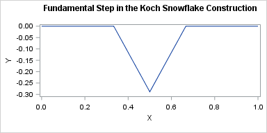
For simplicity, the graph at right shows the first step of the construction on a single line segment that has one endpoint at (0,0) and another endpoint at (1,0). The original horizontal line segment of length one is replaced by four line segments of length 1/3. The first and fourth segments are in the same direction as the original segment (horizontal). The second segment is rotated -60 degrees from the original direction. It, too, is 1/3 the original length. The third segment connects the second and fourth line segments.

The following program defines a function that uses the vector capabilities of SAS/IML software to carry out the fundamental step on a line segment. The function takes two row vectors as arguments, which are the (x,y) coordinates of the endpoints of the line segment. The function returns a 5 x 2 matrix, where the rows contain the endpoints of the four line segments that result from the Koch construction.

Two statements in the function might be unfamiliar. The direct product operator (@) quickly constructs points that are k/3 units along the original line segment for k=0, 1, 2, and 3. The ATAN2 function computes the direction angle for a two-dimensional vector.

proc iml;
/* divide a line segment (2 pts) into 4 segments (5 pts).  
   Create middle point by rotating through -60 degrees */ 
start KochDivide(A, E);                    /* (x,y) coords of endpoints */
   segs = j(5, 2, .);                      /* matrix to hold 4 shorter segs */
   v = (E-A) / 3;                          /* vector 1/3 as long as orig */
   segs[{1 2 4 5}, ] = A + v @ T(0:3);     /* endpoints of new segs */
   /* Now compute middle point. Use ATAN2 to find direction angle. */
   theta = -constant("pi")/3 + atan2(v[2], v[1]); /* change angle by pi/3 */
   w = cos(theta) || sin(theta);           /* vector to middle point */
   segs[3,] = segs[2,] + norm(v)*w;
   return segs;
finish;
 
/* test on line segment from (0,0) to (1,0) */
s = KochDivide({0 0}, {1 0});
title  "Fundamental Step in the Koch Snowflake Construction";
ods graphics / width=600  height=300; 
call series(s[,1], s[,2]) procopt="aspect=0.333";

Construct the Koch snowflake in SAS

Now that we have defined a function that can replace a segment by four shorter segments, let's define a function that applies that function repeatedly to each segment of a polygon. The following function takes two arguments: the polygon and the number of iterations. An N-sided closed polygon is represented as an (N+1) x 2 matrix of vertices.

/* create Koch Snowflake from and equilateral triangle */
start KochPoly(P0, iters=5);    
P = P0;
do j=1 to iters;
   N = nrow(P) - 1;             /* old number of segments */
   newP = j(4*N+1, 2);          /* new number of segments + 1 */
   do i=1 to N;                 /* for each segment... */
      idx = (4*i-3):(4*i+1);                    /* rows for 4 new segments */
      newP[idx, ] = KochDivide(P[i,], P[i+1,]); /* generate new segments */
   end;
   P = newP;                    /* update polygon and iterate */
end;
return P;
finish;

To test the function, define an equilateral triangle. The call to the KochPoly function creates a Koch snowflake from the equilateral triangle.

/* create equilateral triangle as base for snowflake */
pi = constant("pi");
angles = -pi/6 // pi/2 // 7*pi/6;  /* angles for equilateral triangle */
P = cos(angles) || sin(angles);    /* vertices of equilateral triangle */
P = P // P[1,];                    /* append first vertex to close triangle */
K = KochPoly(P);                   /* create the Koch snowflake */

The Koch snowflake that results from this iteration is shown at the top of this article. For completeness, here are the statements that write the snowflake to a SAS data set and graph it by using PROC SGPLOT:

S = j(nrow(K), 3, 1);      /* add ID variable with constant value 1 */
S[ ,1:2] = K;
create Koch from S[colname={X Y ID}];  append from S;  close;
QUIT;
 
ods graphics / width=400px height=400px;
footnote justify=Center "Koch Snowflake";
proc sgplot data=Koch;
   styleattrs wallcolor=CXD6EAF8;               /* light blue */
   polygon x=x y=y ID=ID / outline fill fillattrs=(color=white);
   xaxis display=none;
   yaxis display=none;
run;

Generalizations of the Koch snowflake

The KochPoly function does not check whether the polygon argument is an equilateral triangle. Consequently, use the function to "Koch-ify" any polygon! For example pass in the rectangle with vertices P = {0 0, 2 0, 2 1, 0 1, 0 0}; to create a "Koch box."

Enjoy playing with the program. Let me know if you generate an interesting shape!