Many SAS procedure compute statistics and also compute confidence intervals for the associated parameters. For example, PROC MEANS can compute the estimate of a univariate mean, and you can use the CLM option to get a confidence interval for the population mean. Many parametric regression procedures (such as PROC GLM) can compute confidence intervals for regression parameters. There are many other examples.

If an analysis provides confidence intervals (interval estimates) for multiple parameters, the coverage probabilities apply individually for each parameter. However, sometimes it is useful to construct simultaneous confidence intervals. These are wider intervals for which you can claim that all parameters are in the intervals simultaneously with confidence level 1-α.

This article shows how to use SAS to construct a set of simultaneous confidence intervals for the population mean. The middle of this article uses some advanced multivariate statistics. If you only want to see the final SAS code, jump to the last section of this article.

The distribution of the mean vector

If the data are a random sample from a multivariate normal population, it is well known (see Johnson and Wichern, Applied Multivariate Statistical Analysis, 1992, p. 149; hereafter abbreviated J&W) that the distribution of the sample mean vector is also multivariate normal. There is a multivariate version of the central limit theorem (J&W, p. 152) that says that the mean vector is approximately normally distributed for random samples from any population, provided that the sample size is large enough. This fact can be used to construct simultaneous confidence intervals for the mean.

Recall that the most natural confidence region for a multivariate mean is a confidence ellipse. However, simultaneous confidence intervals are more useful in practice.

Confidence intervals for the mean vector

Before looking at multivariate confidence intervals (CI), recall that many a univariate two-sided CIs are symmetric intervals with endpoints b ± m*SE, where b is the value of the statistic, m is some multiplier, and SE is the standard error of the statistic. The multiplier must be chosen so that the interval has the appropriate coverage probability. For example, the two-sided confidence interval for the univariate mean is has the familiar formula xbar ± t_c SE, where xbar is the sample mean, t_c is the critical value of the t statistic with significance level α and n-1 degrees of freedom, and SE is the standard error of the mean. In SAS, you can compute t_c as quantile("t", 1-alpha/2, n-1).

You can construct similar confidence intervals for the multivariate mean vector. I will show two of the approaches in Johnson and Wichern.

Hotelling T-squared statistic

As shown in the SAS documentation, the radii for the multivariate confidence ellipse for the mean are determined by critical values of an F statistic. The Hotelling T-squared statistic is a scaled version of an F statistic and is used to describe the distribution of the multivariate sample mean.

The following SAS/IML program computes the T-squared statistic for a four-dimensional sample. The Sashelp.iris data contains measurements of the size of petals and sepals for iris flowers. This subset of the data contains 50 observations for the species iris Virginica. (If you don't have SAS/IML software, you can compute the means and standard errors by using PROC MEANS, write them to a SAS data set, and use a DATA step to compute the confidence intervals.)

proc iml;
use sashelp.iris where(species="Virginica"); /* read data */
read all var _NUM_ into X[colname=varNames];
close;
 
n = nrow(X);               /* num obs (assume no missing) */
k = ncol(X);               /* num variables */
alpha = 0.05;              /* significance level */
xbar = mean(X);            /* mean of sample */
stderr = std(X) / sqrt(n); /* standard error of the mean */
 
/* Use T-squared to find simultaneous CIs for mean parameters */
F = quantile("F", 1-alpha, k, n-k);  /* critical value of F(k, n-k) */
T2 = k*(n-1)/(n-k) # F;              /* Hotelling's T-squared is scaled F */
m = sqrt( T2 );                      /* multiplier */
Lower = xbar - m # stdErr;
Upper = xbar + m # stdErr;
T2_CI = (xbar`) || (Lower`) || (Upper`);
print T2_CI[F=8.4 C={"Estimate" "Lower" "Upper"}  R=varNames];

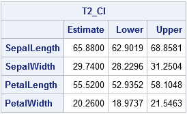
The table shows confidence intervals based on the T-squared statistic. The formula for the multiplier is a k-dimensional version of the 2-dimensional formula that is used to compute confidence ellipses for the mean.

Bonferroni-adjusted confidence intervals

It turns out that the T-squared CIs are conservative, which means that they are wider than they need to be. You can obtain a narrower confidence interval by using a Bonferroni correction to the univariate CI.

The Bonferroni correction is easy to understand. Suppose that you have k MVN mean parameters that you want to cover simultaneously. You can do it by choosing the significance level of each univariate CI to be α/k. Why? Because then the joint probability of all the parameters being covered (assuming independence) will be (1 - α/k)^k, and by Taylor's theorem (1 - α/k)^k ≈ 1 - α when (α/k) is very small. (I've left out many details! See J&W p. 196-199 for the full story.)

In other words, an easy way to construct simultaneous confidence intervals for the mean is to compute the usual two-sided CIs for significance level α/k, as follows:

/* Bonferroni adjustment of t statistic when there are k parameters */
tBonf = quantile("T", 1-alpha/(2*k), n-1);  /* adjusted critical value */
Lower = xbar - tBonf # stdErr;              
Upper = xbar + tBonf # stdErr;
Bonf_CI = (xbar`) || (Lower`) || (Upper`);
print Bonf_CI[F=8.4 C={"Estimate" "Lower" "Upper"} R=varNames];

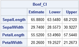
Notice that the confidence intervals for the Bonferroni method are narrower than for the T-square method (J&W, p. 199).

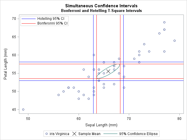
The following graph shows a scatter plot of two of the four variables. The sample mean is marked by an X. For reference, the graph includes a bivariate confidence ellipse. The T-squared confidence intervals are shown in blue. The thinner Bonferroni confidence intervals are shown in red.

Compute simultaneous confidence intervals for the mean in SAS

The previous sections have shown that the Bonferroni method is an easy way to form simultaneous confidence intervals (CIs) for the mean of multivariate data. If you want the overall coverage probability to be at most (1 - α), you can construct k univariate CIs, each with significance level α/k.

You can use the following call to PROC MEANS to construct simultaneous confidence intervals for the multivariate mean. The ALPHA= method enables you to specify the significance level. The method assumes that the data are all nonmissing. If your data contains missing values, use listwise deletion to remove them before computing the simultaneous CIs.

/* Bonferroni simultaneous CIs. For k variables, specify alpha/k 
   on the ALPHA= option. The data should c ontain no missing values. */
proc means data=sashelp.iris(where=(species="Virginica")) nolabels
     alpha=%sysevalf(0.05/4)  /* use alpha/k, where k is number of variables */
     mean clm maxdec=4;
var SepalLength SepalWidth PetalLength PetalWidth;  /* k = 4 */
run;

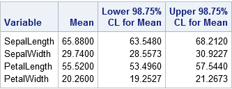
The values in the table are identical to the Bonferroni-adjusted CIs that were computed earlier. The values in the third and fourth columns of the table define a four-dimensional rectangular region. For 95% of the random samples drawn from the population of iris Virginica flowers, the population means will be contained in the regions that are computed in this way.