My previous blog post describes how to implement Conway's Game of Life by using the dynamically linked graphics in SAS/IML Studio. But the Game of Life is not the only kind of cellular automata. This article describes a system of cellular automata that is known as Wolfram's Rule 30. In this blog post I show how to compute and visualize this system in SAS by using traditional PROC IML and a simple heat map.
Wolfram's Rule 30
Conway's Game of Life is a set of rules for evolving cellular automata on a two-dimensional grid. However, one-dimensional automata are simpler to describe and to compute. A well-known one-dimensional example is Wolfram's Rule 30 (1983, Rev. Mod. Phys.). Consider a sequence of binary symbols, such as 0 and 1. An initial configuration determines the next generation by using the following two rules for each cell:
- If the cell and its right-hand neighbor are both 0, then the new value of the cell is the value of its left-hand neighbor.
- Otherwise, the new value of the cell is the opposite of the value of its left-hand neighbor.
The rules are often summarized by using three-term sequences that specify the value of the left, center, and right cells. The sequence 100 means that the center cell is 0, its left neighbor is 1, and its right neighbor is 0. According to the first rule, the value of the center cell for the next generation will be 1. The sequence 000 means that the center cell and both its neighbors are 0. According to the first rule, the value of the center cell for the next generation will be 0. All other sequences are governed by the second rule. For example, the sequence 010 implies that the center cell for the next generation will be 1, which is the opposite of the value of the left neighbor.
There are several ways that you can implement Rule 30 in a matrix language such as SAS/IML. The following SAS/IML program defines a function that returns the next generation of binary values when given the values for the current generation. As for the Game of Life, I define the leftmost and rightmost cells to be neighbors. The evolution function is vectorized, which means that no loops are used to compute a new generation from the previous generation. The second function computes each new generation as a row in a matrix. You can print that matrix or use the HEATDISC subroutine in SAS/IML 13.1 to create a black-and-white heat map of the result.
proc iml;
start Rule30Evolve(x);                     /* x is binary row vector */
   y = x[ncol(X)] || x || x[1];            /* extend x periodically */
   N = ncol(y);
   j = 2:N-1;    xj = y[,j];               /* the original cells */
   R = y[,j+1];  L = y[,j-1];              /* R=right neighbor; L=left neighbor */
   idxSame = loc(xj=0 & R=0);              /* x00 --> center cell is x */
   if ^IsEmpty(idxSame) then y[,idxSame+1] = L[,idxSame];
   idxDiff = setdif(1:N-2, idxSame);       /* otherwise, center cell is ^x */
   if ^IsEmpty(idxDiff) then y[,idxDiff+1] = ^L[,idxDiff];
   return( y[,j] );
finish;

start Rule30(x0, Iters=ceil(ncol(x0)/2));
   N = ncol(x0);
   M = j(Iters,N,0);                       /* initialize array to 0 */
   M[1,] = x0;                             /* set initial configuration */
   do i = 2 to Iters;
      M[i,] = Rule30Evolve(M[i-1,]);       /* put i_th generation into i_th row */
   end;
   return( M );
finish;

N = 101;
x0 = j(1,N,0);                       /* initialize array to 0 */
x0[ceil(N/2)] = 1;                   /* set initial condition for 1st row */
M = Rule30(x0, N);
ods graphics / width=800px height=600px;
call heatmapdisc(M) displayoutlines=0 colorramp={White Black}
title = "Wolfram's Rule 30 (N=101)"; |
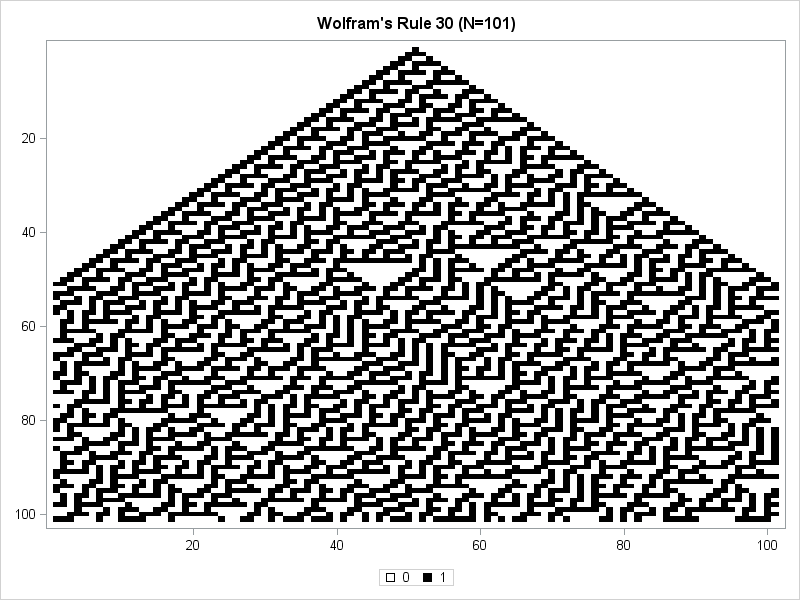
The discrete heat map uses white to indicate cells that are 0 and black to indicate cells that are 1. The initial configuration has 100 cells of white and a single black cell in the middle of the array. That configuration is shown in the first row of the heat map. (Click to enlarge.) The second generation has three black cells in the middle, as shown in the second row. The central region of cells grows two cells larger for each generation. For the first 50 generations, the left boundary is always 001 and the right boundary alternates between 111 and 001. The pattern of the interior cells is not periodic, although certain interesting patterns appear, such as "martini glasses" of various sizes.
After 50 generations, the left and right edges begin to interact in a nontrivial way. Periodicity at the edges is replaced by irregular patterns.
Supposedly the evolution of the middle cell of the array generates nearly random 0-1 values. Mathematica, a computer software package created by Stephen Wolfram, uses the central column of a Rule-30 cellular automata as a random number generator. From a simple deterministic rule comes complex behavior that seems indistinguishable from randomness.
The heat map shows all generations at a single glance by stacking them as rows in a single image. This is different from the Game of Life visualization, which used animation to show how an initial configuration evolves from one generation to the next. You can also use animation to visualize the Rule-30 system. The following animated GIF shows the same 100 generations of an initial configuration that consists of a single black cell in the middle of a 101-cell array. This animation shows how that configuration evolves in time.

It is fun to play with Rule 30. To begin, I suggest an array of 21 cells that evolves for 20 generations. The resulting black-and-white heat map is small enough to study, and you can use the DISPLAYOUTLINES=1 option to better visualize which cells are white during the evolution. You can invent your own initial configuration or use random initial conditions, as shown below:
N = 21;
x0 = T( randfun(N, "Bernoulli", 4/N) );   /* random; expect 4 black cells */
M = Rule30(x0);
call heatmapdisc(M) displayoutlines=1 colorramp={White Black}
title = "Wolfram's Rule 30 (N=21)"; |
Enjoy!

2 Comments
Pingback: Video: Using heat maps to visualize matrices - The DO Loop
Pingback: Pascal’s triangle in SAS - The DO Loop