My last blog post showed how to simulate data for a logistic regression model with two continuous variables. To keep the discussion simple, I simulated a single sample with N observations. However, to obtain the sampling distribution of statistics, you need to generate many samples from the same logistic model. This article shows how to simulate many samples efficiently in the SAS/IML language. The example is from my book Simulating Data with SAS.
The program in my previous post consists of four steps. (Or five, if you count creating a data set as a separate step.) To simulate multiple samples, put a DO loop around Step 4, the step that generates a random binary response vector from the probabilities that were computed for each observation in the model. The following program writes a single data set that contains 100 samples. Each sample is identified by an ordinal variable named SampleID. The data set is in the form required for BY-group processing, which is the efficient way to simulate data with SAS.
%let N = 150;                                     /* N = sample size */
%let NumSamples = 100;                            /* number of samples */
proc iml;
call randseed(1);
X = j(&N, 3, 1);                               /* X[,1] is intercept */
/* 1. Read design matrix for X or assign X randomly.
   For this example, x1 ~ U(0,1) and x2 ~ N(0,2)  */
X[,2] = randfun(&N, "Uniform");
X[,3] = randfun(&N, "Normal", 0, 2);

/* Logistic model with parameters {2, -4, 1} */
beta = {2, -4, 1};
eta = X*beta;                       /* 2. linear model */
mu = logistic(eta);                 /* 3. transform by inverse logit */

/* create output data set. Output data during each loop iteration.     */
varNames = {"SampleID" "y"} || ("x1":"x2");           /* 1st col is ID */
Out = j(&N,1) || X;                /* matrix to store simulated data   */
create LogisticData from Out[c=varNames];
y = j(&N,1);                       /* allocate response vector         */
do i = 1 to &NumSamples;           /* the simulation loop              */
   Out[,1] = i;                         /* update value of SampleID    */
   call randgen(y, "Bernoulli", mu);    /* 4. simulate binary response */
   Out[,2] = y;
   append from Out;                     /* 5. output this sample       */
end;                               /* end loop                         */
close LogisticData;
quit; |
You can call PROC LOGISTIC and specify the SampleID variable on the BY statement. This will produce a set of 100 statistics. The union is an approximate sampling distribution for the statistics. The following call to PROC LOGISTIC computes 100 parameter estimates and saves them to the PE data set.
options nonotes; proc logistic data=LogisticData noprint outest=PE; by SampleId; model y(Event='1') = x1 x2; run; options notes; |
Notice that the call to PROC LOGISTIC uses the NOPRINT option (and the NONOTES option) to suppress unnecessary output during the simulation.
You can use PROC UNIVARIATE to examine the sampling distribution of each parameter estimate. Of course, the parameter estimates also have correlation with each other, so you might also be interested in how the estimates are jointly distributed. You can use the CORR procedure to analyze and visualize the pairwise distributions of the estimates.
In the following statements, I do something slightly more complicated. I use PROC SGSCATTER to create a matrix of pairwise scatter plots of the parameter estimates, with the true parameter values overlaid on the estimates. It requires extra DATA steps to create and merge the parameter values, but I like visualizing the location of the estimates relative to the parameter values. Click on the image to enlarge it.
/* visualize sampling distribution of estimates; overlay parameter values */ data Param; Intercept = 2; x1 = -4; x2 = 1; /* parameter values */ run; data PE2; set PE Param(in=param); /* append parameter values */ if param then Beta = "True Value"; /* add ID variable */ else Beta = "Estimate "; run; ods graphics / reset ATTRPRIORITY=none; title "Parameter Estimates from Logistic Regression"; title2 "&NumSamples Simulated Data Sets, N = &N"; proc sgscatter data=PE2 datasymbols=(Circle StarFilled); matrix Intercept x1 x2 / group=Beta markerattrs=(size=11); run; |
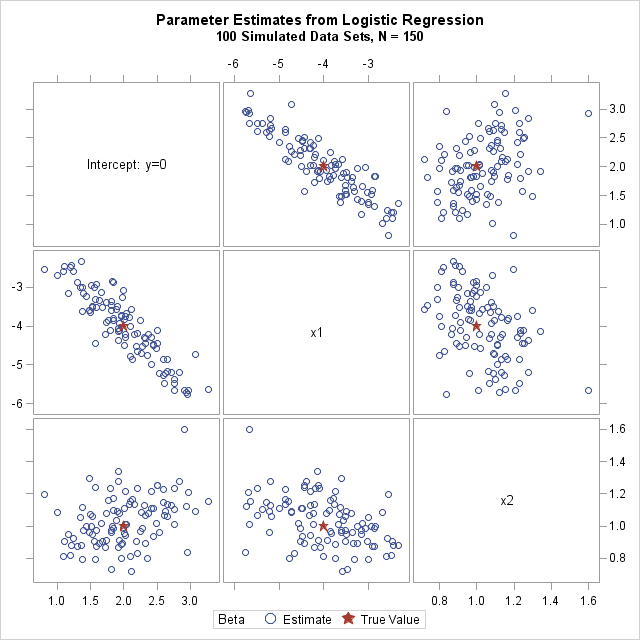
The scatter plot matrix shows pairwise views of the sampling distribution of the three regression coefficients. The graph shows the variability of these estimates in a logistic model with the specified design matrix. It also shows how the coefficients are correlated.
By using the techniques in this post, you can simulate data for other generalized or mixed regression models. You can use similar techniques simulate data from other kinds of multivariate models.

12 Comments
Hello,
I am new to proc iml and i have only come to use it because i need to simulate alot of data. I need proc iml to save all the simulated data sets that i want but i don't know how, i tried to use the reasoning above but its not working. Below is my code,i am simulating 1000 sample datasets. Each with 1800 subjects but the output final dataset i get is only of one dataset.Basically i need proc iml to simulate 1000 sample datasets which i can be able to save and that i can identify by sample ID.
%let nsim=1000;
%macro simulate;
%do i = 1 %to ≁
Proc iml;
beta1=-0.18633;
/***create id matrix***/
id=1:1800;id=id
;
p_id=setdif(id,t_id);p_id=p_id`;
/**treatment allocation***/
trt_1=j(nrow(t_id),1,1);
trt_0=j(nrow(p_id),1,0);
/**combine id with its allocated treatment**/
treat=t_id||trt_1;placebo=p_id||trt_0;
/**append treat and placebo***/
dataset=treat//placebo;
do k=1 to nrow(dataset);
time_i=0; status=0;recurr_sub={};
do until (time_i>1.5);
/**create an empty vector and fill it with generated survival times**/
x=j(1,1,.);
call randseed(123);
call randgen(x,'uniform');
linpred=exp(beta1*dataset[k,2]);
study_time=-log(x)/(0.55*linpred);
time_i=study_time + time_i;
if time_i<=1.5 then status=1;else status=0;
/***extract and combine id,treat,survival times,recurrence status***/
idd=dataset[k,1]; trt=dataset[k,2];
row_sub=idd||trt||study_time||status||time_i;
/***binding rows for events**/
recurr_sub=recurr_sub//row_sub;
end;
/***combine all subjects***/
allsub=allsub//recurr_sub;
end;
create aom from allsub[colname={"id" "treat" "survtime" "status" "cumutime"}];
append from allsub;
create main_data from dataset[colname={"id" "treat"}];
append from dataset;
%end;
%mend simulate;
%simulate;
run;
Here are some suggestions:
1) Since you are new to SAS/IML, read about tips for learning the SAS/IML language
2) The SAS/IML language already has loops, so you rarely need to use macro loops with SAS/IML. Read this article on why macro loops in simulation are inefficient.
3) Use the techniques in my book Simulating Data with SAS to write a single SAS data set that contains all of the data.
4) If you have specific programming questions, ask them at the SAS/IML Support Community.
5) For efficiency, avoid looping over all rows and avoid dynamically growing a vector in a loop (by using concatenation). For more tips, see "Eight tips to make your simulation run faster," especially #1, #3, and the Note at the end.
Hello Rick,
Would it at all be possible to have a similar code in SAS/STAT, since I do not have SAS/IML ? If so, how do you propose it can be done ? Thanks a lot !
Regards,
Jack
This example uses uncorrelated explanatory variables, so yes it is possible to run this example in the DATA step. (Using the DATA step to simulate correlated explanatory variables is more challenging.) There are examples in Chapters 11 and 12 of my book Simulating Data with SAS.
Hi,
Nice post indeed.
Why does the intercept is more correlated with x1 than with x2?
An excellent question! I was hoping that someone would notice that. The x1 variable is uniform on [0,1], so it is always positive. In contrast, the x2 variable is normally distributed, which means it is (approximately) centered. The fact that x1 is not centered means that it is more correlated with the intercept. If you change the definition of x1 to use normal data, then the correlations with the intercept are approximately the same magnitude. If you center the x1 data (uniform - 0.5), then the correlation between x1 and the intercept is not as strong.
How to control the prevalence of outcome, Y? Using the above code, 50% observation got Y = 1. However, I want Y = 1 for 5%, 10% and 20% of observations.
I found one way to do this - make change in step 4 as follows.
/* call randgen(y, "Bernoulli", 0.10); * / -- This will give Y=1 for 10% of obs.
However, this will also lead to random generation of Y and the discrimination of model will be 0.5 which makes model not useful. Is that correct?
Your statement is correct, but your model no longer depends on the covariates. The correct way to do it is to adjust the vector of coefficients, beta.
Pingback: Simulating data for a logistic regression model - The DO Loop
Pingback: Simulate data for a linear regression model - The DO Loop
Hello,
If I have generated a dataset, how do I use such to run 1000 logistic regressions and save predicted probabilities for each?
As mentioned in this article, use the BY statement to analyze the 1000 logistic regressions. Use the OUTPUT statement with the PREDICTED= option to output the predicted probabilities.