In my book Simulating Data with SAS, I show how to use the SAS DATA step to simulate data from a logistic regression model. Recently there have been discussions on the SAS/IML Support Community about simulating logistic data by using the SAS/IML language. This article describes how to efficiently simulate logistic data in SAS/IML, and is based on the DATA step example in my book.
The SAS documentation for the LOGISTIC procedure includes a brief discussion of the mathematics of logistic regression. To simulate logistic data, you need to do the following:
- Assign the design matrix (X) of the explanatory variables. This step is done once. It establishes the values of the explanatory variables in the (simulated) study.
- Compute the linear predictor, η = X β, where β is a vector of parameters. The parameters are the "true values" of the regression coefficients.
- Transform the linear predictor by the logistic (inverse logit) function. The transformed values are in the range (0,1) and represent probabilities for each observation of the explanatory variables.
- Simulate a binary response vector from the Bernoulli distribution, where each 0/1 response is randomly generated according to the specified probabilities from Step 3.
Presumably you are simulating the data so that you can call PROC LOGISTIC and obtain parameter estimates and other statistics for the simulated data. So, optionally, Step 5 is to write the data to a SAS data set so that PROC LOGISTIC can read it. Here's a SAS/IML program that generates a single data set of 150 simulated observations:
/* Example from _Simulating Data with SAS_, p. 226--229 */
%let N = 150;                                     /* N = sample size */
proc iml;
call randseed(1);
X = j(&N, 3, 1);                               /* X[,1] is intercept */
/* 1. Read design matrix for X or assign X randomly.
   For this example, x1 ~ U(0,1) and x2 ~ N(0,2)  */
X[,2] = randfun(&N, "Uniform");
X[,3] = randfun(&N, "Normal", 0, 2);

/* Logistic model with parameters {2, -4, 1} */
beta = {2, -4, 1};
eta = X*beta;                       /* 2. linear model */
mu = logistic(eta);                 /* 3. transform by inverse logit */

/* 4. Simulate binary response. Notice that the
      "probability of success" is a vector (SAS/IML 12.1)            */
y = j(&N,1);                             /* allocate response vector */
call randgen(y, "Bernoulli", mu);        /* simulate binary response */

/* 5. Write y and x1-x2 to data set*/
varNames = "y" || ("x1":"x2");
Out = X; Out[,1] = y;            /* simulated response in 1st column */
create LogisticData from Out[c=varNames];  /* no data is written yet */
append from Out;                               /* output this sample */
close LogisticData;
quit; |
The SAS/IML statements for simulating logistic data are concise. A few comments on the program:
- The design matrix contains two continuous variables. In this simulation, one is uniformly distributed; the other is normally distributed. This was done for convenience. You could also read in a data set that defines the observed values of the explanatory variables. See the discussion and examples in Simulating Data with SAS, p. 201–205. (Notice also that I used the RANDFUN function in SAS/IML 12.3 to generate these variables.)
- The linear model does not contain an error term, as would be the case for linear regression. Instead, the binary response is random because we called the RANDGEN subroutine to generate a Bernoulli random variable.
- The parameter to the Bernoulli distribution is a vector of probabilities. This feature requires SAS/IML 12.1.
- So that the program can be extended to support an arbitrary number of explanatory variables, I copy all of the numerical data into the Out matrix, which is a copy of the X matrix except that the intercept column is replaced by the simulated binary responses. This matrix is written to a SAS data set.
What do the simulated data look like? The following call to SGPLOT produces a scatter plot of the X1 and X2 variables, with "events" colored red and "non-events" colored blue:
proc sgplot data=LogisticData; scatter x=x1 y=x2 / group=y markerattrs=(symbol=CircleFilled); run; |
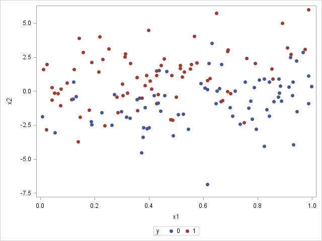
The graph shows that the probability of an event decreases as you move from X1=0 (where there are many red markers) to X1=1 (where there are few red markers). This makes sense because the model coefficient for X1 is negative. In contrast, the probability of an event increases as you move from negative values of X2 to positive values. This makes sense because the model coefficient for X2 is positive. In general, most events (red markers) are in the upper left portion of the graph, whereas most non-events (blue markers) are in the lower right portion.
For small samples, there is a lot of uncertainty in the parameter estimates for a logistic regression. In this example, 150 observations were generated so that you can run PROC LOGISTIC against the simulated data and see that the parameter estimates are close to the parameter values. The following statement uses the CLMPARM=WALD option to compute parameter estimates and confidence intervals for the parameters:
proc logistic data=LogisticData plots(only)=Effect; model y(Event='1') = x1 x2 / clparm=wald; ods select CLParmWald EffectPlot; run; |
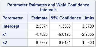
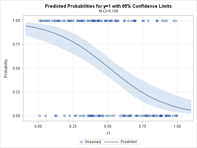
Notice that the parameter estimates are somewhat close to the parameter values of (2, -4, 1). The 95% confidence intervals include the parameter values. (Re-run the program with N = 1000 or N = 10000 to see whether the estimates get closer to the parameters!) The graph shows the predicted probability of an event as a function of X1, conditioned on X2=0.1, which is the mean value of X2. You could request a similar plot for the predicted probability as a function of X2 (at the mean of X1) by using the option
plots(only)=Effect(showobs X=(X1 X2));
This article shows how to generate a single sample of data that fits a logistic regression model. My next blog post shows how to generalize this program to efficiently simulate and analyze many samples.

18 Comments
Hi Rick-- Nice post! We covered this from the data step perspective, and in R, in http://sas-and-r.blogspot.com/2009/06/example-72-simulate-data-from-logistic.html back in 2009, and revisit it this week in thinking about interactions: http://sas-and-r.blogspot.com/2014/06/example-20147-simulate-logistic.html
Pingback: Simulate many samples from a logistic regression model - The DO Loop
Pingback: Simulating data for a logistic regression model in Excel | Nathan Brixius
How do I simulate an extra X3 categorical variable (say with 5 categories) for the same model
Use the Table distribution to simulate categorical data in SAS.
Thanks
Very useful simulation example! I have a question, Rick. What is the difference between RANDFUN and RANDGEN functions? A similar question is related to the logistic reg simulation in Simulating Data using SAS book; an array has been created and the array was filled using do loop and RAND function. I wrote a similar code and generated numbers with and without array. There doesn't seem to be a difference. Is it a matter of efficiency or values should be generated one at a time?
In the DATA step, use RAND, which is a function. In SAS/IML you have a choice. The RANDGEN subroutine is more efficient and should be used insode of loops. The RANDFUN function is more convenient. For more details, see "Convenient functions vs efficient subroutines."
Thanks Rick!
What will be the form of the logit function if Y is a binary variable such that y=0 with probability p and y=1 with probability (1-p).
Thanks
logit(1-p)
How we can interpret the estimated regression parameter (β) resulted from the regression model in terms of odds rato if y is a binary variable such that y=0 with probability p and y=1 with probability (1-p).
Thanks
The interpretation of the betas is the usual interpretation, except the "event" is Y=0. These questions are best asked on a discussion forum. You can try the SAS Statistical Procedures Community or StackOverflow.
Thanks for your help. You mentioned that. The interpretation of the betas is the usual interpretation, except the "event" is Y=0. Does it mean if the estimated value of β=2, then the odds of being in the category y=0 is doubled for a unit increase in X?
Yes, provided that X is a continuous regressor and that the other variables in the model are held constant, the difference in the log-odds changes by 2.
Provided that X is a continuous regressor and that the other variables in the model are held constant,if the estimated value of β=2, then the odds ratio=7.4. Can we explain it as if x increases by one unit, then it is more likely that y=0?
Thanks
Thank you for all these questions. As I've said several times, this is not the right place for them. I cannot provide personal support for statistical questions. If you have a question or comment about something in the blog, please post it here and I will respond. However, if you have a general question about staistics or SAS programming, please use the Support Communities.
Thank you.