In a previous article I discussed how to bin univariate observations by using the BIN function, which was added to the SAS/IML language in SAS/IML 9.3. You can generalize that example and bin bivariate or multivariate data. Over two years ago I wrote a blog post on 2D binning in the SAS/IML language, but that post was written before the SAS/IML 9.3 release, so it does not take advantage of the BIN function.
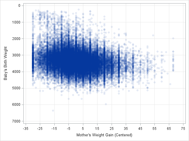
The image to the left shows a scatter plot of data from the Sashelp.BWeight data set. For 50,000 pregnancies, the birth weight of the baby (in grams) is plotted against the weight gain of the mother (in pounds), adjusted so that the median weight gain is centered at zero. There are 11 subintervals in the horizontal direction and seven subintervals in the vertical direction. Consequently, there are 77 cells, which you can enumerate in row-major order beginning with the upper-left cell.
A two-dimensional binning of these data enables you to find the bin for each observation. Many statistics use binned data. For example, you can do a chi-square test for association, estimate density, and test for spatial randomness. The following SAS/IML statements associates a bin number to each observation. The Bin2D function calls the BIN function twice.
proc iml;
use sashelp.bweight;
read all var {m_wtgain weight} into Z;  /* SAS 9.4: Use {MomWtGain Weight} */
close;

/* define two-dimensional binning function */
start Bin2D(u, cutX, cutY);
   bX = bin(u[,1], cutX);   /* bins in X direction: 1,2,...,kx */
   bY = bin(u[,2], cutY);   /* bins in Y direction: 1,2,...,ky */
   bin = bX + (ncol(cutX)-1)*(bY-1);     /* bins 1,2,...,kx*ky */
   return(bin);
finish;

cutX = do(-35, 75, 10);            /* cut points in X direction */
cutY = do(0, 7000, 1000);          /* cut points in Y direction */
b = Bin2D(Z, cutX, cutY); /* bin numbers 1-77 */ |
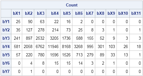
I wrote the Bin2D function to return an index, but you can convert the index into a subscript if you prefer. (For example, the index 77 corresponds to the subscript (11, 7).) The index is useful for tabulating the number of observations in each bin. The TABULATE call counts the number of observations in each bin, which you can visualize by forming a frequency table:
call tabulate(binNumber, Freq, b);           /* count in each bin */
Count = j(ncol(cutY)-1, ncol(cutX)-1, 0);    /* allocate matrix */
Count[binNumber] = Freq;                     /* fill nonzero counts */
print Count[c=('bX1':'bX11') r=('bY1':'bY7')]; |
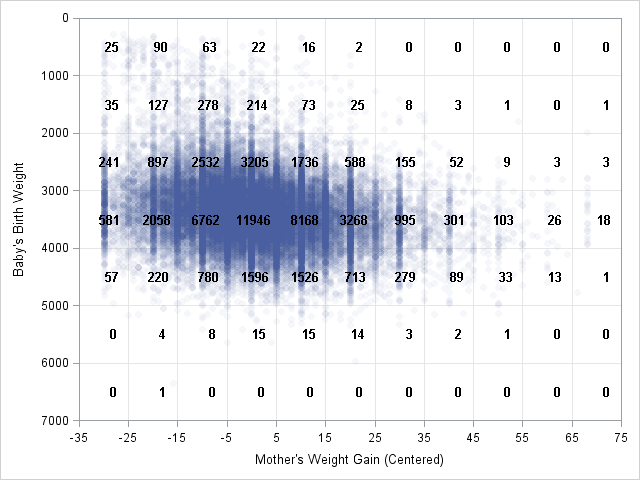
Notice that the Y axis is reversed on the scatter plot. This makes it easy to compare the scatter plot and the tabular frequencies.
If you want to overlay the frequencies on the scatter plot, you can write the cell counts to a SAS data set and use PROC SGPLOT. The result is shown in the following figure. You can download the program used to create the figures in this blog post.
In summary, you can use the BIN function in the SAS/IML language to bin data in many dimensions. The BIN function is simpler than using the DATA step or PROC FORMAT. It handles unevenly spaced intervals and semi-infinite intervals. It's also fast. So next time you you want to group continuous data into intervals—or higher-dimensional cells!— give it a try.

2 Comments
Pingback: Counting observations in two-dimensional bins - The DO Loop
Pingback: Designing a quantile bin plot - The DO Loop