The power of a statistical test measures the test's ability to detect a specific alternate hypothesis. For example, educational researchers might want to compare the mean scores of boys and girls on a standardized test. They plan to use the well-known two-sample t test. The null hypothesis is that the means of the two groups are equal. Will the t test be able to detect a difference in the two group means (if it exists) by rejecting the null hypothesis?
The ability to detect differences in the group means depends on the sample sizes in the study, but it is safe to say that the t test is unlikely to detect small differences in the students' mean scores, and it is more likely to detect larger differences.
In general, the power of a test is the probability that the test will reject the null hypothesis when a specified alternative is true. For the t test, power means the probability that the test can detect a mean difference of a specified magnitude. In general, this can be a difficult computation because it requires knowing the sampling distribution of the test statistic under the alternative hypothesis. For simple tests (such as the two-sample t test), the sampling distribution is known, but for more complicated statistical tests the power computation might be available only by using simulation methods.
This article describes how to use simulation to estimate the power of the t test. For this simple test, we can check the simulation by using the exact answer, as provided by the POWER procedure in SAS. However, the simulation will illustrate general ideas that you can use to estimate the power of more complicated statistical tests. This article is based on material in Chapter 5 of Simulating Data with SAS.
Formulation of the problem
In this simulation, I assume that each population is normally distributed. For simplicity, assume the population for Group 1 is N(0, 1) and the population for Group 2 is N(δ, 1), where δ > 0 is the difference between the population means.
The null hypothesis for the t test is that δ = 0. Given two samples, the t test will either reject the null hypothesis at the α = 0.05 significance level or it won't. In the simulation approach, you simulate many samples, and estimate the probability of rejecting the null hypothesis by using the empirical proportion of simulated samples that rejected the null hypothesis. (This uses the law of large numbers.)
The following steps estimate the power for the two-sample pooled t test:
- Simulate data from the model for each group's population. These are the samples. The populations are chosen so that the true difference between the population means is δ > 0. (The null hypothesis is false.)
- Run the TTEST procedure on the samples. For each sample, record whether the t test rejects the null hypothesis.
- Count how many times the t test rejects the null hypothesis. This proportion is an estimate for the power of the test.
Simulating the data
The following SAS statements define parameters for the simulation and use the DATA step to simulate 5,000 simulated trials. All of the data are in a single data set, and the SampleID variable identifies which observations belong to which simulated trial. In this simulation, each group has 10 observations and the true difference between the population means is 1.2, which is a little larger than the standard deviations of the populations.
%let n1 = 10; /* group sizes*/ %let n2 = 10; %let NumSamples = 5000; /* number of simulated samples */ %let Delta = 1.2; /* true size of mean difference in population */ data PowerSim(drop=i); call streaminit(321); do SampleID = 1 to &NumSamples; do i = 1 to &n1; c=1; x = rand("Normal", 0, 1); /* Group 1: x ~ N(0,1) */ output; end; do i = 1 to &n2; c=2; x = rand("Normal", &Delta, 1); /* Group 2: x ~ N(Delta, 1) */ output; end; end; run; |
Analyzing the Simulated Data
As I have written previously, use BY-group processing to carry out efficient simulation and analysis in SAS. Also, be sure to suppress the display of tables and graphs during the analysis by using the the %ODSoff and macro. The following SAS statements define the %ODSOff and %ODSOn macros, and analyze all data for the simulated trials:
%macro ODSOff(); /* Call prior to BY-group processing */ ods graphics off; ods exclude all; ods noresults; %mend; %macro ODSOn(); /* Call after BY-group processing */ ods graphics on; ods exclude none; ods results; %mend; /* 2. Compute (pooled) t test for each sample */ %ODSOff proc ttest data=PowerSim; by SampleID; class c; var x; ods output ttests=TTests(where=(method="Pooled")); run; %ODSOn |
The TTEST procedure creates an output data set that contains 5,000 rows, one for each simulated trial. The data set includes a variable named Probt, which gives the result of the t test on each trial.
Count the rejections to estimate power
The last step in the simulation is to estimate the power, which is the probability of rejecting the null hypothesis. The following SAS statements create an indicator variable that has the value 1 if the t test rejected the null hypothesis at the 0.05 significance level, and the value 0 otherwise. (Alternatively, you could define a SAS format.) You can then use PROC FREQ to count the proportion of trials for which the t test rejected the null hypothesis.
/* Construct indicator var for obs that reject H0 at 0.05 significance */ data Results; set TTests; RejectH0 = (Probt <= 0.05); run; /* 3. Compute proportion: (# that reject H0)/NumSamples and CI */ proc freq data=Results; tables RejectH0 / nocum binomial(level='1'); run; |
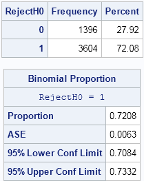
The FREQ procedure indicates that the power of the two-sample t test is about 72%. The 95% confidence interval for that estimate is [0.708, 0.733]. This estimate is for the scenario of samples of sizes 10, where one sample is drawn from N(0,1) and the other is drawn from N(1.2, 1).
As mentioned earlier, you can use PROC POWER to find the exact power for the two-sample t test, as follows:
proc power; twosamplemeans power = . /* missing ==> "compute this" */ meandiff=1.2 stddev=1 ntotal=20; /* 20 obs in the two samples */ run; |
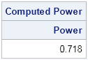
The estimate from the simulation is very close to the true power of the t test.
Next week I will extend this simulation to estimate points along a power curve.

17 Comments
Pingback: Using simulation to compute a power curve - The DO Loop
Hi Rick,
My question is for onesamplemeans application of proc power (like the example below). Can you point me to references for the theoretical formula that proc power uses for the confidence interval precision. Thanks! -Richard
http://support.sas.com/documentation/cdl/en/statug/63033/HTML/default/viewer.htm#statug_power_sect022.htm
The formula is in the section Confidence Interval for Mean (CI=T) The end of the chapter has a References section, if you need a published reference.
Hi Rick,
I'm working on computing the power of the Gehan test (a generalization of the Wilcoxon Rank-Sum Test, for censored data). I need to generate two samples of the same size from two normal distributions [e.g. N(mean,std) and N(mean+loc,std)], where both samples have left-censored values, with the same amount of censoring in each group, and in such a way that the same censoring distribution [e.g. U(min,max)] is used in both groups. I’m using PROC IML for this purpose, and I'm comparing the values generated from the normal distributions with the values generated from the uniform distribution, and I censor a normal value whenever it is smaller than a uniform value, and I consider the normal value to be uncensored if it is greater than the uniform value; however, due to the sample sizes and censoring restrictions in each group, I'm throwing out some of the normal values whenever they don't satisfy all my criteria, and I don't think this is perfect solution, since it will bias some of the values in the two samples. Do you have any suggestion on how to generate data that satisfy all these criteria, and without throwing out some of the values generated from the sequence of random normal values?
Thank you, Daniel.
First. I think that Gehan's test is supported by PROC POWER, so you don't actually need the simulation (or you can use PROC POWER to check simulation results). Second, are you claiming that you need the same number of censored values in the two groups? That seems strange since if the means differ, I would expect one group to have more censoring. I would double check the assumptions of the test. I would expect that you can generate N1 N(mu,sigma)obs from group 1, of which k1 are censored, and then generate N2 N(mu+delta,sigma) from group 2, of which k2 are censored. If you disagree, I suggest posting your question to the SAS statistical procedures community.
Pingback: 13 popular articles from 2013 - The DO Loop
Dear Rick,
thank you so much for this blog! I hope you can help me with a very similar issue: I wrote a similar program to verify the proc power results for an equivalence test, but something must be wrong:
proc power;
twosamplemeans
test=equiv_diff
meandiff=0
lower=-0.05
upper=0.05
stddev=0.1
alpha=0.05
power=0.80
npergroup=.;
run;
This results in N=70 per group.
I then run 1000 simulations with these sample size of 2 x 70:
%let S=1000;
%let N=70;
data Sim;
do t=1 to &S;
do p=1 to &N;
Trt='Drug'; C=rand('normal',0,0.1); output;
Trt='Comp'; C=rand('normal',0,0.1); output;
end;
end;
run;
proc ttest data=Sim test=diff tost(-0.05, 0.05);
by t;
class trt;
var C;
ods output EquivLimits=Equiv;
run;
proc freq data=Equiv;
where method='Pooled';
table Assessment;
run;
I'd expect to see ca. 5% of ' Not equivalent' in the last table, corresponding to the alpha level, but in fact it is about 17%. Where is my error in reasoning?
Thanks!
Andi
You can ask questions like this at the SAS Support Communities. Posting to that site enables many people to offer suggestions, and the site supports uploading files that contain programs, data, etc.
17% is approximately 20%, and that is what this simulation should show because you are simulating the power of the test (P(reject H0| H1 is true)) when N=70. Look at the first few observations of the EQUIV data set and you will see that PROC TTEST is asking whether a certain confidence interval about the sample mean is entirely within the interval [-0.05, 0.05]. The value of alpha determines the width of the CI.
Rick,
Do you have some examples for using simulation to compare actual vs. nominal Test Size?
Thanks,
-Richard
Yes. In my book you can look at the examples that discuss "coverage probaility." The approach is similar to estimating power: simulate many draws from data that satisfy the null hypothesis, run the test on each sample, count the proportion of times that the test rejected the null hypothesis.
I want to find the power of the Gail-Simon test. How can I use proc power for that?
I don't know about PROC POWER, but it seems like you can follow the basic outline of this article to simulate the power curve: Simulate the data and run PROC FREQ, but include the CMH(GAILSIMON) option in the TABLES statement. If you have further questions, post them to the SAS Support Communities.
Hi Rick:
Using SAS bootstrap, do you have any suggestions of how to create data sets that show a specified difference with same standard error between two groups by creating virtual subjects that reflect random draws from a normal distribution. Then create 1000 virtual trials where you sample 50 from each and estimate the treatment difference?
This sounds like an ANOVA simulation, or possibly a GLM if there are continuous covariates. See the topic "Simulate many samples from a linear regression model." If you have further questions, post the program you are trying to write (even if it doesn't work) to one of the SAS Support Communities.
Hi Rick,
I am really struggling to do a sample size calculation for 3x3 cross over study with 3 different treatments (placebo, treatment1, treatment2) and an outcome variable that is a continuous one. and normally distributed.
Could you please point me to a working code to use?
Very much appreciate your help. I have already asked for help in SAS communities but couldn't really get an answer.
The SAS Support Community is the right place to ask that question. I do not know the answer.