In a recent article on efficient simulation from a truncated distribution, I wrote some SAS/IML code that used the LOC function to find and exclude observations that satisfy some criterion. Some readers came up with an alternative algorithm that uses the REMOVE function instead of subscripts. I remarked in a comment that it is interesting to compare the relative efficiency of matrix subscripts and the REMOVE function, and that Chapter 15 of my book Statistical Programming with SAS/IML Software provides a comparison. This article uses the TIME function to measure the relative performance of each method.
The task we will examine is as follows: given a vector x and a value x0, return a row vector that contains the values of x that are greater than x0. The following two SAS/IML functions return the same result, but one uses the REMOVE function whereas the other uses the LOC function and subscript extraction:
proc iml;
/* 1. Use REMOVE function, which supports empty indices */
start Test_Remove(x, x0);
   return( (remove(x, loc(x<=x0))) );
finish;

/* 2. Use subscripts, which do not support empty indices */
start Test_Substr(x, x0);
   idx = loc(x>x0);          /* find all less than values */
   if ncol(idx)>0 then
      return( T(x[idx]) );   /* return less than values */
   else return( idx );       /* return empty matrix */
finish; |
To test the relative performance of the two functions, create a vector x that contains one million normal variates. By using the QUANTILE function, you can obtain various cut points so that approximately 1%, 5%, 10%,...,95%, and 99% of the values will be truncated when you call the functions:
/* simulate 1 million random normal variates */
call randseed(1);
N = 1e6;
x = j(N,1);
call randgen(x, "Normal");

/* compute normal quantiles so fncs return about 1%, 5%,...,95%, 99% of x */
prob = 0.01 || do(0.05,0.95,0.05) || 0.99;
q = quantile("Normal", 1-prob); |
The following loop calls each function 50 times and computes the average time for the function to return the truncated data. The results of using the REMOVE function are stored in the first column of the results matrix. The second column stores the results of using index subscripts.
NRepl = 50;      /* repeat computations this many times */
results = j(ncol(prob),2);

do i = 1 to ncol(prob);
   t0 = time();
   do k = 1 to NRepl;
      y = Test_Remove(x, q[i]);
   end;
   results[i,1] = time()-t0;

   t0 = time();
   do k = 1 to NRepl;
      z = Test_Substr(x, q[i]);
   end;
   results[i,2] = time()-t0;
end;
results = results / NRepl; /* average time */ |
You can use the SGPLOT procedure to plot the time that each function takes to extract 1%, 5%, ..., 95%, and 99% of data. In addition, you can smooth the performance by using a loess curve:
/* stack vertically and add categorical variable */
Method = j(ncol(Prob), 1, "Remove") // j(ncol(Prob), 1, "Subscripts");
Time = results[,1] // results[,2];
Prob = Prob` // Prob`;
create Timing var {"Prob" "Method" "Time"};  append;  close Timing;

title "Average Time to Truncate One Million Observations";
proc sgplot data=Timing;
   loess x=Prob y=Time / group = Method;
   yaxis label="Average Time (s)";
   xaxis label="Probability of Truncation";
run; |
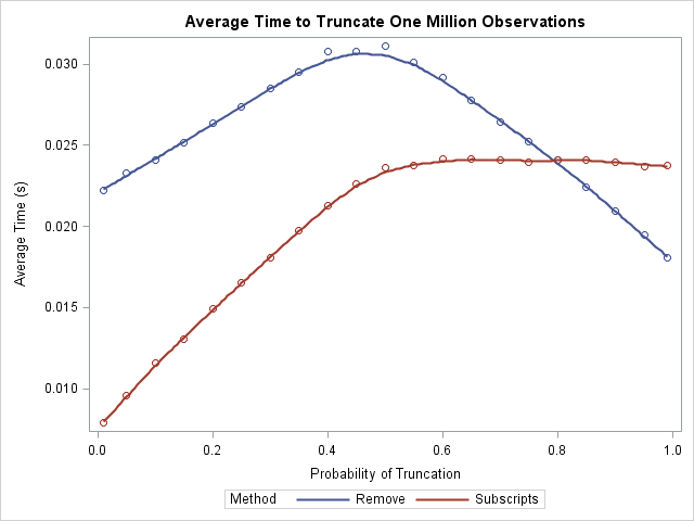
What does this exercise tell us? First, notice that the average time for either algorithm is a few hundredths of a second, and this is for a vector that contains a million elements. This implies that, in practical terms, it doesn't matter which algorithm you choose! However, for people who care about algorithmic performance, the LOC-subscript algorithm outperforms the REMOVE function provided that you truncate less than 80% of the observations. When you truncate 80% or more, the REMOVE function has a slight advantage.
Notice the interesting shapes of the two curves. The REMOVE algorithm performs worse when 50% of the points are truncated. The LOC-subscript function is faster when fewer than 50% of the points are truncated, and then levels out. There is essentially no difference in performance between 50% truncation and 99% truncation.
The value in this article is not in analyzing the performance of these particular algorithms. Rather, the value is in knowing how to use the TIME function to compare the performance of whatever algorithms you encounter. That programming skill comes in handy time and time again.

6 Comments
That's really interesting Rick. I am finding it hard to understand the flatness of the red line. Intuitively the time the subscription process x[idx] takes must increase linearly with the length of the vector idx. So for the line to be flat, it must be the case that the syntax loc(x>x0) is taking less time to run when it returns longer and longer idx vectors (above 0.5 on the chart). Does that make sense from your understanding of the algorithm behind the LOC function?
Yes, it is an interesting graph! If you time the LOC function by itself, it looks like the graph of the REMOVE function: it goes up, reaches a peak at prob=0.5, then goes down. As you say, if you time the subscript operation by itself, it increases linearly. Consequently, the superposition flattens out, as you see.
As to why the LOC function requires LESS time when it returns a LONGER vector, my conjecture is that it is because of the way that computer cache works. Even though the function has to copy MORE values, it is cheap to copy a value that is already in the cache. For long vectors, it is very probable that observation (i+1) is in the cache, given that observation i is in the cache. So the LOC function experiences fewer cache misses in this case.
Does anyone have a competing theory? If so, post your ideas.
Pingback: An efficient way to increment a matrix diagonal - The DO Loop
Pingback: Excluding variables: Read all but one variable into a matrix - The DO Loop
Pingback: Jackknife estimates in SAS - The DO Loop
Pingback: 6 tips for timing the performance of algorithms - The DO Loop